Binomial and Poisson Distribution (Applet)

Open Applet in new Tab

Applet Description

This applet allows the calculation and graphical display of

the probabilities ${\rm Pr}(z=\mu)$ of a discrete random variable $z \in \{\mu \} = \{0, 1, 2, 3, \text{...} \}$, that determine its Probability Density Function (PDF) – here representation with Dirac functions ${\rm \delta}( z-\mu)$:

$$f_{z}(z)=\sum_{\mu=1}^{M}{\rm Pr}(z=\mu)\cdot {\rm \delta}( z-\mu),$$

the probabilities ${\rm Pr}(z \le \mu)$ of the Cumulative Distribution Function (CDF):

$$F_{z}(\mu)={\rm Pr}(z\le\mu).$$

Discrete distributions are available in two sets of parameters:

the Binomial distribution with the parameters $I$ and $p$ ⇒ $z \in \{0, 1, \text{...} \ , I \}$ ⇒ $M = I+1$ possible values,
the Poisson distribution with the parameter $\lambda$ ⇒ $z \in \{0, 1, 2, 3, \text{...}\}$ ⇒ $M \to \infty$.

In the exercises below you will be able to compare:

two Binomial distributions with different sets of parameters $I$ and $p$,
two Poisson distributions with different rates $\lambda$,
a Binomial distribution with a Poisson distribution.

Theoretical Background

Properties of the Binomial Distribution

The Binomial distribution represents an important special case for the likelihood of occurence of a discrete random variable. For the derivation we assume, that $I$ binary and statistically independent random variables $b_i \in \{0, 1 \}$ can take

the value $1$ with the probability ${\rm Pr}(b_i = 1) = p$, and
the value $0$ with the probability ${\rm Pr}(b_i = 0) = 1-p$.

The sum

$$z=\sum_{i=1}^{I}b_i$$

is also a discrete random variable with symbols from the set $\{0, 1, 2, \cdots\ , I\}$ with size $M = I + 1$ and is called "binomially distributed".

Probabilities of the Binomial Distribution

The probabilities to find $z = \mu$ for $μ = 0, \text{...}\ , I$ are given as

$$p_\mu = {\rm Pr}(z=\mu)={I \choose \mu}\cdot p^\mu\cdot ({\rm 1}-p)^{I-\mu},$$

with the number of combinations $(I \text{ over }\mu)$:

$${I \choose \mu}=\frac{I !}{\mu !\cdot (I-\mu) !}=\frac{ {I\cdot (I- 1) \cdot \ \cdots \ \cdot (I-\mu+ 1)} }{ 1\cdot 2\cdot \ \cdots \ \cdot \mu}.$$

Moments of the Binomial Distribution

Consider a binomially distributed random variable $z$ and its expected value of order $k$:

$$m_k={\rm E}[z^k]=\sum_{\mu={\rm 0}}^{I}\mu^k\cdot{I \choose \mu}\cdot p^\mu\cdot ({\rm 1}-p)^{I-\mu}.$$

We can derive the formulas for

the linear average: $m_1 = I\cdot p,$
the quadratic average: $m_2 = (I^2-I)\cdot p^2+I\cdot p,$
the variance and standard deviation: $\sigma^2 = {m_2 - m_1^2} = {I \cdot p\cdot (1-p)} \hspace{0.3cm}\Rightarrow \hspace{0.3cm} \sigma = \sqrt{I \cdot p\cdot (1-p)}.$

Applications of the Binomial Distribution

The Binomial distribution has a variety of uses in telecommunications as well as in other disciplines:

It characterizes the distribution of rejected parts (Ausschussstücken) in statistical quality control.
The simulated bit error rate of a digital transmission system is technically a binomially distributed random variable.
The binomial distribution can be used to calculate the residual error probability with blockwise coding, as the following example shows.

$\text{Example 1:}$ When transfering blocks of $I =5$ binary symbols through a channel, that

distorts a symbol with probability $p = 0.1$ ⇒ random variable $e_i = 1$, and
transfers the symbol undistorted with probability $1 - p = 0.9$ ⇒ random variable $e_i = 0$,

the new random variable $f$ („Error per block”) calculates to:

$$f=\sum_{i=1}^{I}e_i.$$

$f$ can now take integer values between $\mu = 0$ (all symbols are correct) and $\mu = I = 5$ (all five symbols are erroneous). We describe the probability of $\mu$ errors as $p_μ = {\rm Pr}(f = \mu)$.

The case that all five symbols are transmitted correctly occurs with the probability of $p_0 = 0.9^{5} ≈ 0.5905$. This can also be seen from the binomial formula for $μ = 0$ , considering the definition $5\text{ over } 0 = 1$.
A single error $(f = 1)$ occurs with the probability $p_1 = 5\cdot 0.1\cdot 0.9^4\approx 0.3281$. The first factor indicates, that there are $5\text{ over } 1 = 5$ possibe error positions. The other two factors take into account, that one symbol was erroneous and the other four are correct when $f =1$.
For $f =2$ there are $5\text{ over } 2 = (5 \cdot 4)/(1 \cdot 2) = 10$ combinations and you get a probability of $p_2 = 10\cdot 0.1^2\cdot 0.9^3\approx 0.0729$.

If a block code can correct up to two errors, the residual error probability is $p_{\rm R} = 1-p_{\rm 0}-p_{\rm 1}-p_{\rm 2}\approx 0.85\%$. A second calculation option would be $p_{\rm R} = p_{3} + p_{4} + p_{5}$ with the approximation $p_{\rm R} \approx p_{3} = 0.81\%.$

The average number of errors in a block is $m_f = 5 \cdot 0.1 = 0.5$ and the variance of the random variable $f$ is $\sigma_f^2 = 5 \cdot 0.1 \cdot 0.9= 0.45$ ⇒ standard deviation $\sigma_f \approx 0.671.$

Properties of the Poisson Distribution

The Poisson distribution is a special case of the Binomial distribution, where

$I → \infty$ and $p →0$.
Additionally, the parameter $λ = I · p$ must be finite.

The parameter $λ$ indicates the average number of "ones" in a specified time unit and is called rate.

Unlike the Binomial distribution where $0 ≤ μ ≤ I$, here, the random variable can assume arbitrarily large non-negative integers, which means that the number of possible values is not countable. However, since no intermediate values can occur, the Poisson distribution is still a "discrete distribution".

Probabilities of the Poisson Distribution

With the limits $I → \infty$ and $p →0$, the likelihood of occurence of the Poisson distributed random variable $z$ can be derived from the probabilities of the Binomial distribution:

$$p_\mu = {\rm Pr} ( z=\mu ) = \lim_{I\to\infty} \cdot \frac{I !}{\mu ! \cdot (I-\mu )!} \cdot (\frac{\lambda}{I} )^\mu \cdot ( 1-\frac{\lambda}{I})^{I-\mu}.$$

After some algebraic transformations we finally obtain

$$p_\mu = \frac{ \lambda^\mu}{\mu!}\cdot {\rm e}^{-\lambda}.$$

Moments of the Poisson Distribution

The moments of the Poisson distribution can be derived directly from the corresponding equations of the Binomial distribution by taking the limits again:

$$m_1 =\lim_{\left.{I\hspace{0.05cm}\to\hspace{0.05cm}\infty, \hspace{0.2cm} {p\hspace{0.05cm}\to\hspace{0.05cm} 0}}\right.} \hspace{0.2cm} I \cdot p= \lambda,\hspace{0.8cm} \sigma =\lim_{\left.{I\hspace{0.05cm}\to\hspace{0.05cm}\infty, \hspace{0.2cm} {p\hspace{0.05cm}\to\hspace{0.05cm} 0}}\right.} \hspace{0.2cm} \sqrt{I \cdot p \cdot (1-p)} = \sqrt {\lambda}.$$

We can see that for the Poisson distribution $\sigma^2 = m_1 = \lambda$ always holds. In contrast, the moments of the Binomial distribution always fulfill $\sigma^2 < m_1$.

rechts

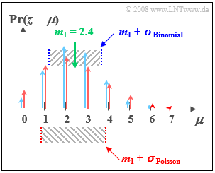
$\text{Example 2:}$ We now compare the Binomial distribution with parameters $I =6$ und $p = 0.4$ with the Poisson distribution with $λ = 2.4$:

Both distributions have the same linear average $m_1 = 2.4$.
The standard deviation of the Poisson distribution (marked red in the figure) is $σ ≈ 1.55$.
The standard deviation of the Binomial distribution (marked blue) is $σ = 1.2$.

Applications of the Poisson Distribution

The Poisson distribution is the result of a so-called Poisson point process which is often used as a model for a series of events that may occur at random times. Examples of such events are

failure of devices - an important task in reliability theory,
shot noise in the optical transmission simulations, and
the start of conversations in a telephone relay center („Teletraffic engineering”).

$\text{Example 3:}$ A telephone relay receives ninety requests per minute on average $(λ = 1.5 \text{ per second})$. The probabilities $p_µ$, that in an arbitrarily large time frame exactly $\mu$ requests are received, is:

$$p_\mu = \frac{1.5^\mu}{\mu!}\cdot {\rm e}^{-1.5}.$$

The resulting numerical values are $p_0 = 0.223$, $p_1 = 0.335$, $p_2 = 0.251$, etc.

From this, additional parameters can be derived:

The distance $τ$ between two requests satisfies the "exponential distribution",
The mean time span between two requests is ${\rm E}[τ] = 1/λ ≈ 0.667 \ \rm s$.

Comparison of Binomial and Poisson Distribution

This section deals with the similarities and differences between Binomial and Poisson distributions.

Binomial vs. Poisson distribution

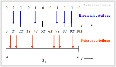
The Binomial distribution is used to describe stochastic events, that have a fixed period $T$. For example the period of an ISDN (Integrated Services Digital Network) network with $64 \ \rm kbit/s$ is $T \approx 15.6 \ \rm \mu s$.

Binary events such as the error-free $(e_i = 0)$/ faulty $(e_i = 1)$ transmission of individual symbols only occur in this time frame.
With the Binomial distribution, it is possible to make statistical statements about the number of expected erros in a period $T_{\rm I} = I · T$, as is shown in the time figure above (marked blue).
For very large values of $I$ and very small values of $p$, the Binomial distribution can be approximated by the Poisson distribution with rate $\lambda = I \cdot p$.
If at the same time $I · p \gg 1$, the Poisson distribution as well as the Binomial distribution turn into a discrete Gaussian distribution according to the de Moivre-Laplace Theorem.

The Poisson distribution can also be used to make statements about the number of occuring binary events in a finite time interval.

By assuming the same observation period $T_{\rm I}$ and increasing the number of partial periods $I$, the period $T$, in which a new event ($0$ or $1$) can occur, gets smaller and smaller. In the limit where $T$ goes to zero, this means:

With the Poisson distribution binary events can not only occur at certain given times, but at any time, which is illustrated in the second time chart.
In order to get the same number of "ones" in the period $T_{\rm I}$ - in average - as in the Binomial distribution (six pulses in the example), the characteristic probability $p = {\rm Pr}( e_i = 1)$ for an infinitesimal small time interval $T$ must go to zero.

Exercises

In these exercises, the term Blue refers to distribution function 1 (marked blue in the applet) and the term Red refers to distribution function 2 (marked red in applet).

(1) Set Blue to Binomial distribution $(I=5, \ p=0.4)$ and Red to Binomial distribution $(I=10, \ p=0.2)$.

What are the probabilities ${\rm Pr}(z=0)$ and ${\rm Pr}(z=1)$?

$\hspace{1.0cm}\Rightarrow\hspace{0.3cm}\text{Blue: }{\rm Pr}(z=0)=0.6^5=7.78\%, \hspace{0.3cm}{\rm Pr}(z=1)=0.4 \cdot 0.6^4=25.92\%;$

$\hspace{1.85cm}\text{Red: }{\rm Pr}(z=0)=0.8^{10}=10.74\%, \hspace{0.3cm}{\rm Pr}(z=1)=0.2 \cdot 0.8^9=26.84\%.$

(2) Using the same settings as in (1), what are the probabilities ${\rm Pr}(3 \le z \le 5)$?

$\hspace{1.0cm}\Rightarrow\hspace{0.3cm}\text{Note that }{\rm Pr}(3 \le z \le 5) = {\rm Pr}(z=3) + {\rm Pr}(z=4) + {\rm Pr}(z=5)\text{, or } {\rm Pr}(3 \le z \le 5) = {\rm Pr}(z \le 5) - {\rm Pr}(z \le 2)$

$\hspace{1.85cm}\text{Blue: }{\rm Pr}(3 \le z \le 5) = 0.2304+ 0.0768 + 0.0102 =1 - 0.6826 = 0.3174;$

$\hspace{1.85cm}\text{Red: }{\rm Pr}(3 \le z \le 5) = 0.2013 + 0.0881 + 0.0264 = 0.9936 - 0.6778 = 0.3158.$

(3) Using the same settings as in (1), what are the differences in the linear average $m_1$ and the standard deviation $\sigma$ between the two Binomial distributions?

$\hspace{1.0cm}\Rightarrow\hspace{0.3cm}\text{Average:}\hspace{0.2cm}m_\text{1} = I \cdot p\hspace{0.3cm} \Rightarrow\hspace{0.3cm} m_\text{1, Blue} = 5 \cdot 0.4\underline{ = 2 =} \ m_\text{1, Red} = 10 \cdot 0.2; $

$\hspace{1.85cm}\text{Standard deviation:}\hspace{0.4cm}\sigma = \sqrt{I \cdot p \cdot (1-p)} = \sqrt{m_1 \cdot (1-p)}\hspace{0.3cm}\Rightarrow\hspace{0.3cm} \sigma_{\rm Blue} = \sqrt{2 \cdot 0.6} =1.095 < \sigma_{\rm Red} = \sqrt{2 \cdot 0.8} = 1.265.$

(4) Set Blue to Binomial distribution $(I=15, p=0.3)$ and Red to Poisson distribution $(\lambda=4.5)$.

What differences arise between both distributions regarding the average $m_1$ and variance $\sigma^2$?

$\hspace{1.0cm}\Rightarrow\hspace{0.3cm}\text{Both distributions have the same average:}\hspace{0.2cm}m_\text{1, Blue} = I \cdot p\ = 15 \cdot 0.3\hspace{0.15cm}\underline{ = 4.5 =} \ m_\text{1, Red} = \lambda$;

$\hspace{1.85cm} \text{Binomial distribution: }\hspace{0.2cm} \sigma_\text{Blue}^2 = m_\text{1, Blue} \cdot (1-p)\hspace{0.15cm}\underline { = 3.15} < \text{Poisson distribution: }\hspace{0.2cm} \sigma_\text{Red}^2 = \lambda\hspace{0.15cm}\underline { = 4.5}$;

(5) Using the same settings as in (4), what are the probabilities ${\rm Pr}(z \gt 10)$ and ${\rm Pr}(z \gt 15)$?

$\hspace{1.0cm}\Rightarrow\hspace{0.3cm} \text{Binomial: }\hspace{0.2cm} {\rm Pr}(z \gt 10) = 1 - {\rm Pr}(z \le 10) = 1 - 0.9993 = 0.0007;\hspace{0.3cm} {\rm Pr}(z \gt 15) = 0 \ {\rm (exactly)}$.

$\hspace{1.85cm}\text{Poisson: }\hspace{0.2cm} {\rm Pr}(z \gt 10) = 1 - 0.9933 = 0.0067;\hspace{0.3cm}{\rm Pr}(z \gt 15) \gt 0\hspace{0.2cm}( \approx 0)$;

$\hspace{1.85cm}\text{Approximation: }\hspace{0.2cm}{\rm Pr}(z \gt 15) \ge {\rm Pr}(z = 16) = \lambda^{16} /{16!}\approx 2 \cdot 10^{-22}$

(6) Using the same settings as in (4), which parameters lead to a symmetric distribution around $m_1$?

$\hspace{1.0cm}\Rightarrow\hspace{0.3cm} \text{Binomial distribution with }p = 0.5\text{: }p_\mu = {\rm Pr}(z = \mu)\text{ symmetric around } m_1 = I/2 = 7.5 \ ⇒ \ p_μ = p_{I–μ}\ ⇒ \ p_8 = p_7, \ p_9 = p_6, \text{etc.}$

$\hspace{1.85cm}\text{In contrast, the Poisson distribution is never symmetric, since it extends to infinity!}$

Zur Handhabung des Applets

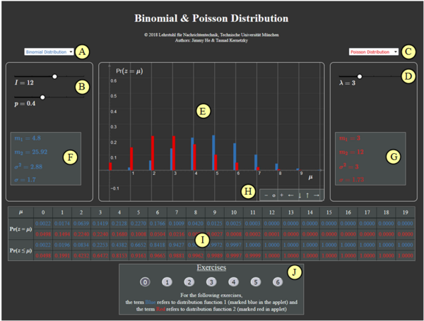
(A) Vorauswahl für blauen Parametersatz

(B) Parametereingabe $I$ und $p$ per Slider

(C) Vorauswahl für roten Parametersatz

(D) Parametereingabe $\lambda$ per Slider

(E) Graphische Darstellung der Verteilungen

(F) Momentenausgabe für blauen Parametersatz

(G) Momentenausgabe für roten Parametersatz

(H) Variation der grafischen Darstellung

$\hspace{1.5cm}$„$+$” (Vergrößern),

$\hspace{1.5cm}$ „$-$” (Verkleinern)

$\hspace{1.5cm}$ „$\rm o$” (Zurücksetzen)

$\hspace{1.5cm}$ „$\leftarrow$” (Verschieben nach links), usw.

( I ) Ausgabe von ${\rm Pr} (z = \mu)$ und ${\rm Pr} (z \le \mu)$

(J) Bereich für die Versuchsdurchführung

Andere Möglichkeiten zur Variation der grafischen Darstellung:

Gedrückte Shifttaste und Scrollen: Zoomen im Koordinatensystem,
Gedrückte Shifttaste und linke Maustaste: Verschieben des Koordinatensystems.

About the Authors

This interactive calculation was designed and realized at the Lehrstuhl für Nachrichtentechnik of the Technische Universität München.

The original version was created in 2003 byJi Li as part of her Diploma thesis using „FlashMX–Actionscript” (Supervisor: Günter Söder).
In 2018 this Applet was redesigned and updated to "HTML5" by Jimmy He as part of his Bachelor's thesis (Supervisor: Tasnád Kernetzky) .

Once again: Open Applet in new Tab