Exponentially Distributed Random Variables

One-sided exponential distribution

$\text{Definition:}$ A continuous random variable $x$ is called (one-sided) exponentially distributed if it can take only non–negative values and the PDF for $x>0$ has the following shape:

$f_x(x)=\it \lambda\cdot\rm e^{\it -\lambda \hspace{0.05cm}\cdot \hspace{0.03cm} x}.$

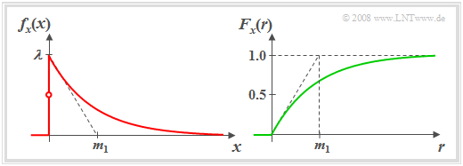
PDF and CDF of an exponentially distributed random variable

The left sketch shows the "probability density function" $\rm (PDF)$ of such an exponentially distributed random variable $x$ . Highlight:

The larger the distribution parameter $λ$ is, the steeper the decay occurs.
By definition $f_{x}(0) = λ/2$ , i.e. the mean of left-hand limit $(0)$ and right-hand limit $(\lambda)$ .

For the "cumulative distribution function" $\rm (CDF)$ , we obtain for $r > 0$ by integration over the PDF (right graph):

$F_{x}(r)=1-\rm e^{\it -\lambda\hspace{0.05cm}\cdot \hspace{0.03cm} r}.$

The "moments" of the one-sided exponential distribution are generally equal to

$m_k = k!/λ^k.$

From this and from Steiner's theorem,nbsp; we get for the "mean"nbsp; and thenbsp; "rms value" (ornbsp; "standard deviation"):

$m_1={1}/{\lambda},$

$\sigma=\sqrt{m_2-m_1^2}=\sqrt{\frac{2}{\lambda^2}-\frac{1}{\lambda^2}}={1}/{\lambda}.$

$\text{Example 1:}$ The exponential distribution has great importance for reliability studies, and the term "lifetime distribution" is also commonly used in this context.

In these applications, the random variable is often the time $t$ that elapses before a component fails.
Furthermore, it should be noted that the exponential distribution is closely related to the Poisson distribution.

Transformation of random variables

To generate such an exponentially distributed random variable on a digital computer, you can use e.g. a nonlinear transformation. The underlying principle is first stated here in general terms.

$\text{Procedure:}$ If a continuous valued random variable $u$ possesses the PDF $f_{u}(u)$ , then the probability density function of the random variable transformed at the nonlinear characteristic $x = g(u)$ holds:

$f_{x}(x)=\frac{f_u(u)}{\mid g\hspace{0.05cm}'(u)\mid}\Bigg \vert_{\hspace{0.1cm} u=h(x)}.$

Here, $g\hspace{0.05cm}'(u)$ denotes the derivative of the characteristic curve $g(u)$ and $h(x)$ gives the inverse function to $g(u)$ .

However, the above equation is only valid under the condition that the derivative $g\hspace{0.03cm}'(u) \ne 0$ .
For a characteristic with horizontal sections $(g\hspace{0.05cm}'(u) = 0)$ : Additional Dirac delta functions appear in the PDF if the input variable has components in these ranges.
The weights of these Dirac functions are equal to the probabilities that the input variable lies in these ranges.

To transform random variables

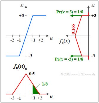
$\text{Example 2:}$ Given a random variable $u$ triangularly distributed between $-2$ and $+2$ on a nonlinearity with characteristic $x = g(u)$ ,

which, in the range $\vert u \vert ≤ 1$ triples the input values, and
mapping all values $\vert u \vert > 1$ to $x = \pm 3$ depending on the sign,

then the PDF $f_{x}(x)$ sketched on the right is obtained.

Please note:

Due to the amplification by a factor of $3$ ⇒ $f_{x}(x)$ is wider and lower than $f_{u}(u)$ by this factor.
The two horizontal limits of the characteristic at $u = ±1$ lead to two Dirac delta functions at $x = ±3$ , each with weight $1/8$ .
The weight $1/8$ corresponds to the green areas in the PDF $f_{u}(u).$

Generation of an exponentially distributed random variable

$\text{Procedure:}$ Now we assume that the random variable $u$ to be transformed is uniformly distributed between $0$ (inclusive) and $1$ (exclusive).

Moreover, we consider the monotonically increasing characteristic curve

$x=g_1(u) =\frac{1}{\lambda}\cdot \rm ln \ (\frac{1}{1-\it u}).$

It can be shown that by this characteristic $x=g_1(u)$ a one-sided exponentially distributed random variable $x$ with the following PDF arises
(derivation see next page):

$f_{x}(x)=\lambda\cdot\rm e^{\it -\lambda \hspace{0.05cm}\cdot \hspace{0.03cm} x}\hspace{0.2cm}{\rm for}\hspace{0.2cm} {\it x}>0.$

For $x = 0$ the PDF value is half $(\lambda/2)$ .
Negative $x$ values do not occur because for $0 ≤ u < 1$ the argument of the (natural) logarithm function does not become smaller than $1$ .

By the way, the same PDF is obtained with the monotonically decreasing characteristic curve

$x=g_2(u)=\frac{1}{\lambda}\cdot \rm ln \ (\frac{1}{\it u})=-\frac{1}{\lambda}\cdot \rm ln(\it u \rm ).$

Please note:

When using a computer implementation corresponding to the first transformation characteristic $x=g_1(u)$ the value $u = 1$ must be excluded.
If one uses the second transformation characteristic $x=g_2(u)$ , on the other hand, the value $u =0$ must be excluded.

The (German) learning video Erzeugung einer Exponentialverteilung $\Rightarrow$ Generation of an exponential distribution, shall clarify the transformations derived here.

Derivation of the corresponding transformation characteristic

$\text{Exercise:}$ Now derive the transformation characteristic $x = g_1(u)= g(u)$ already used on the last page, which is derived from a random variable equally distributed between $0$ and $1$ ; $u$ with the probability density function (PDF) $f_{u}(u)$ forms a one-sided exponentially distributed random variable $x$ with the PDF $f_{x}(x)$ :

$f_{u}(u)= \left\{ \begin{array}{*{2}{c} } 1 & \rm if\hspace{0.3cm} 0 < {\it u} < 1,\\ 0.5 & \rm if\hspace{0.3cm} {\it u} = 0, {\it u} = 1,\ 0 & \rm else, \end{array} \right. \hspace{0.5cm}\rightarrow \hspace{0.5cm} f_{x}(x)= \left\{ \begin{array}{*{2}{c} } \lambda\cdot\rm e^{\it -\lambda\hspace{0.03cm} \cdot \hspace{0.03cm} x} & \rm if\hspace{0.3cm} {\it x} > 0,\ \lambda/2 & \rm if\hspace{0.3cm} {\it x} = 0 ,\ 0 & \rm if\hspace{0.3cm} {\it x} < 0. \ \end{array} \right.$

$\text{Solution:}$

(1) Starting from the general transformation equation.

$f_{x}(x)=\frac{f_{u}(u)}{\mid g\hspace{0.05cm}'(u) \mid }\Bigg \vert _{\hspace{0.1cm} u=h(x)}$

is obtained by converting and substituting the given PDF $f_{ x}(x):$

$\mid g\hspace{0.05cm}'(u)\mid\hspace{0.1cm}=\frac{f_{u}(u)}{f_{x}(x)}\Bigg \vert _{\hspace{0.1cm} x=g(u)}= {1}/{\lambda} \cdot {\rm e}^{\lambda \hspace{0.05cm}\cdot \hspace{0.05cm}g(u)}.$

Here $x = g\hspace{0.05cm}'(u)$ gives the derivative of the characteristic curve, which we assume to be monotonically increasing.

(2) With this assumption we get $\vert g\hspace{0.05cm}'(u)\vert = g\hspace{0.05cm}'(u) = {\rm d}x/{\rm d}u$ and the differential equation ${\rm d}u = \lambda\ \cdot {\rm e}^{-\lambda \hspace{0.05cm}\cdot \hspace{0.05cm} x}\, {\rm d}x$ with solution $u = K - {\rm e}^{-\lambda \hspace{0.05cm}\cdot \hspace{0.05cm} x}.$

(3) From the condition that the input variable $u =0$ should lead to the output value $x =0$ , we obtain for the constant $K =1$ and thus $u = 1- {\rm e}^{-\lambda \hspace{0.05cm}\cdot \hspace{0.05cm} x}.$

(4) Solving this equation for $x$ yields the equation given in front:

$x = g_1(u)= \frac{1}{\lambda} \cdot {\rm ln} \left(\frac{1}{1 - u} \right) .$

In a computer implementation, however, ensure that the critical value $1$ is excluded for the equally distributed input variable $u$
This, however, has (almost) no effect on the final result.

Two-sided exponential distribution - Laplace distribution

Closely related to the exponential distribution is the so-called Laplace distrubtion with the probability density function

$f_{x}(x)=\frac{\lambda}{2}\cdot\rm e^{\it -\lambda \hspace{0.05cm} \cdot \hspace{0.05cm} | x|}.$

The Laplace distribution is a two-sided exponential distribution that approximates sufficiently well, in particular, the amplitude distribution of speech– and music signals.

The moments $k$ –th order ⇒ $m_k$ of the Laplace distribution agree with those of the exponential distribution for even $k$ .
For odd $k$ on the other hand, the (symmetric) Laplace distribution always yields $m_k= 0$ .

For generation one uses a between $±1$ equally distributed random variable $v$ (where $v = 0$ must be excluded) and the transformation characteristic curve

$x=\frac{{\rm sign}(v)}{\lambda}\cdot \rm ln(\it v \rm ).$

Further notes:

From the Exercise 3.8 one can see further properties of the Laplace distribution.

In the (German) learning video Wahrscheinlichkeit und WDF $\Rightarrow$ Probability and PDF, it is shown which meaning the Laplace distribution has for the description of speech– and music signals.
With the applet PDF, CDF and Moments you can display the characteristics $($ PDF, CDF, Moments $)$ of exponential and Laplace distributions.
We also refer you to the applet Two-dimensional Laplace random quantities .

Exercises for the chapter

Exercise 3.8: Amplification and Limitation

Exercise 3.8Z: Circle (Ring) Area

Exercise 3.9: Characteristic Curve for Cosine PDF

Exercise 3.9Z: Sine Transformation