Exercise 3.13: Threshold Decision vs. DFE vs. Maximum Likelihood

Bitte diese Aufgabe sehr genau kontrollieren. Da habe ich etliche Änderungen vorgenommen.

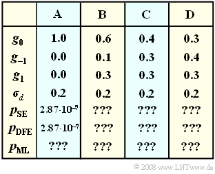
Error probabilities in comparison:
$\bullet$ Threshold Decision $\rm (SE)$,
$\bullet$ Decision Feedback Equalization $\text{(DFE)}$,
$\bullet$ Maximum Likelihood Detection $\text{(ML)}$

Error probabilities of different receiver types are to be compared. Considered are:

Threshold Decision $($German: "Schwellenwertentscheidung" ⇒ "$\rm SE$"$)$ ⇒ error probability $p_{\rm SE}$,
Decision Feedback Equalization $\rm (DFE)$ ⇒ error probability $p_{\rm DFE}$ and
Maximum Likelihood Detection $\rm (ML)$ ⇒ error probability $p_{\rm ML}$.

In the table given are for KORREKTUR: ohne 'for' four different parameter sets $\rm A$, $\rm B$, $\rm C$ and $\rm D$:

The "main value" $g_0$ of the basic detection pulse,
the "precursor" $g_{\rm –1}$,
the "postcursor" (trailer) $g_1$,
the rms value $\sigma_d$ of the detection noise component $d_{\rm N}(t)$ before the respective decision.

Bipolar amplitude coefficients are assumed, so that, for example, for the worst-case error probability $($German: "ungünstigste Fehlerwahrscheinlichkeit" ⇒ "$\rm U$"$)$ of the receiver with threshold decision, the following applies:

$$p_{\rm U,\hspace{0.15cm} SE } = \left\{ \begin{array}{c} {\rm Q}\big [ ({g_0-|g_{-1}|-|g_{1}|})/{\sigma_d} \big ]\\ \\{\rm Q}(0) = 0.5 \end{array} \right.\quad \begin{array}{*{1}c} {\rm with }\hspace{0.15cm}{\rm open }\hspace{0.15cm}{\rm eye }, \\ \\{\rm with }\hspace{0.15cm}{\rm closed }\hspace{0.15cm}{\rm eye }. \\ \end{array}\begin{array}{*{20}c} \\ \end{array}$$

For the Nyquist system $\rm A$, the mean error probability is exactly the same, viz.

$$p_{\rm SE } =p_{\rm U,\hspace{0.15cm} SE } = {\rm Q}\left( {g_0}/{\sigma_d} \right)= {\rm Q}(5) \approx 2.87 \cdot 10^{-7}\hspace{0.05cm}.$$

For the other system variants $\rm B$, $\rm C$ and $\rm D$ considered here, the intersymbol interferences are so strong and the given noise rms value is so small that the following approximation can be applied:

$$p_{\rm SE } \approx {1}/{4} \cdot p_{\rm U,\hspace{0.1cm} SE } = {1}/{4} \cdot {\rm Q}\left( \frac {{\rm Max }\hspace{0.05cm}\big [0, \hspace{0.05cm}g_0-|g_{-1}|-|g_{1}|\big ]}{\sigma_d} \right)\hspace{0.05cm}.$$

Except for the Nyquist system $\rm A$ $($here $p_{\rm DFE} = p_{\rm SE})$, the following approximation applies to the DFE receiver instead:

$$p_{\rm DFE } \approx {1}/{2} \cdot p_{\rm U,\hspace{0.1cm} DFE } = {1}/{2} \cdot {\rm Q}\left( \frac{{\rm Max }\hspace{0.05cm}\big [0, \hspace{0.05cm}g_0-|g_{-1}|\big ]}{\sigma_d} \right)\hspace{0.05cm}.$$

In contrast, it was shown in the "last theory section" for this chapter that for a receiver with ML decision, the following approximation holds:

$$p_{\rm ML } = {\rm Q}\left( \frac{{\rm Max }\hspace{0.05cm}[g_{\nu}]}{\sigma_d} \right)\hspace{0.05cm}.$$

Notes:

The exercise belongs to the chapter "Viterbi Receiver".

Reference is also made to the chapters "Linear Nyquist Equalization" and "Decision Feedback".

You can determine the numerical values of the Q-function using the interaction module "Complementary Gaussian Error Functions".

To apply the algorithm given in the theory section for two precursors, you would have to make the following renamings
$($which, however, has no meaning for the calculation of the error probabilities$)$:

$$g_{1 }\hspace{0.1cm}\Rightarrow \hspace{0.1cm}g_{0 },\hspace{0.4cm} g_{0 }\hspace{0.1cm}\Rightarrow \hspace{0.1cm}g_{-1 },\hspace{0.4cm} g_{-1 }\hspace{0.1cm}\Rightarrow \hspace{0.1cm}g_{-2 } \hspace{0.05cm}.$$

Questions

$\hspace{0.2cm} p_{\rm ML} \ = \ $

$\ \cdot 10^{\rm –7} $

$\hspace{0.25cm} p_{\rm SE} \ = \ $

$\ \% $

$p_{\rm DFE} \ = \ $

$\ \% $

$\hspace{0.2cm} p_{\rm ML} \ = \ $

$\ \% $

$\hspace{0.25cm} p_{\rm SE} \ = \ $

$\ \% $

$p_{\rm DFE} \ = \ $

$\ \% $

$\hspace{0.2cm} p_{\rm ML} \ = \ $

$\ \% $

$\hspace{0.25cm} p_{\rm SE} \ = \ $

$\ \% $

$p_{\rm DFE} \ = \ $

$\ \% $

$\hspace{0.2cm} p_{\rm ML} \ = \ $

$\ \% $

Solution

(1) Without intersymbol interference $\text{(system A)}$, the DFE and ML receivers do not improve over the simple threshold decision:

$$ p_{\rm DFE } = p_{\rm ML } = p_{\rm SE } \hspace{0.15cm}\underline {\approx 2.87 \cdot 10^{-7}} \hspace{0.05cm}.$$

(2) With $g_0 = 0.6$, $g_{\rm –1} = 0.1$ and $g_1 = 0.3$, $\text{(system B)}$, one obtains approximately:

$$p_{\rm SE } \ \approx \ {1}/{4} \cdot {\rm Q}\left( \frac{0.6-0.1-0.3}{0.2} \right)= {1}/{4} \cdot{\rm Q}(1) \hspace{0.15cm}\underline {\approx 4\% \hspace{0.05cm}},$$

$$ p_{\rm DFE } \ \approx \ {1}/{2} \cdot {\rm Q}\left( \frac{0.6-0.1}{0.2} \right)= {1}/{2} \cdot {\rm Q}(2.5) \hspace{0.15cm}\underline {\approx 0.31\%} \hspace{0.05cm},$$

$$ p_{\rm ML } \ \approx \ {\rm Q}\left( \frac{0.6}{0.2} \right) = {\rm Q}(3) \hspace{0.15cm}\underline {\approx 0.135\%} \hspace{0.05cm}.$$

(3) With $g_0 = 0.4$ and $g_1 = g_{\rm –1} = 0.3$ $\text{(system C)}$, one obtains approximately:

$$p_{\rm SE } \ \approx \ {1}/{4} \cdot{\rm Q}(0) \hspace{0.15cm}\underline {= 12.5\%} \hspace{0.3cm}\Rightarrow \hspace{0.3cm}{\rm closed }\hspace{0.15cm}{\rm eye } \hspace{0.05cm},$$

$$ p_{\rm DFE } \ \approx \ {1}/{2} \cdot {\rm Q}\left( \frac{0.4-0.3}{0.2} \right)= {1}/{2} \cdot {\rm Q}(0.5) \hspace{0.15cm}\underline {\approx 15\% \hspace{0.05cm}},$$

$$ p_{\rm ML } \ \approx \ {\rm Q}\left( \frac{0.4}{0.2} \right) = {\rm Q}(2) \hspace{0.15cm}\underline {\approx 2.27\%} \hspace{0.05cm}.$$

Interesting is – and not a calculation error – that the DFE is worse than the conventional threshold decision when the error probability is $10\%$ or more.
See also the solution for subtask (4).

(4) With system $\text{D}$, the DFE receiver also has a closed eye.

$p_{\rm DFE}$ is greater than $p_{\rm SE}$, since the worst-case symbol sequence now occurs more frequently. According to the given simple approximation holds:

$$p_{\rm SE } = {1}/{4} \cdot{\rm Q}(0) = 0.125\hspace{0.05cm}, \hspace{0.2cm} p_{\rm DFE } = {1}/{2} \cdot{\rm Q}(0) \hspace{0.15cm}\underline {= 0.250} \hspace{0.05cm}.$$

On the other hand, with an exact calculation one obtains:

$$p_{\rm SE } \ = \ {1}/{4} \cdot {\rm Q}\left( \frac{0.3-0.4-0.3}{0.2}\right) + {1}/{4} \cdot{\rm Q}\left( \frac{0.3-0.4+0.3}{0.2}\right)+ \ {1}/{4} \cdot {\rm Q}\left( \frac{0.3+0.4-0.3}{0.2}\right) +{1}/{4} \cdot{\rm Q}\left( \frac{0.3+0.4+0.3}{0.2}\right)$$

$$ \Rightarrow \hspace{0.3cm}p_{\rm SE } \ = \ {1}/{4} \cdot \left[ {\rm Q}(-2) + {\rm Q}(1) +{\rm Q}(2) +{\rm Q}(5) \right] ={1}/{4} \cdot \left[ 1+ {\rm Q}(1) +{\rm Q}(5) \right] \hspace{0.05cm}.$$

Because of ${\rm Q}(–2) + {\rm Q}(2) = 1$ and ${\rm Q}(5) \approx 0$ we obtain $p_{\rm SE} \approx 25.5\%$.

The same applies to the DFE receiver:

$$p_{\rm DFE } \ = \ {1}/{2} \cdot {\rm Q}\left( \frac{0.3-0.4}{0.2}\right) + {1}/{2} \cdot{\rm Q}\left( \frac{0.3+0.4}{0.2}\right)= \ {1}/{2} \cdot \left[ {\rm Q}(-0.5) + {\rm Q}(3.5) \right] \approx\frac{1- {\rm Q}(0.5)}{2}\hspace{0.15cm}\underline {= 35\%} \hspace{0.05cm}.$$

In contrast, the error probability $p_{\rm ML}$ of a maximum likelihood receiver is still ${\rm Q}(2) \hspace{0.15cm} \underline {= 2.27\%}$.

The order of the basic detection pulse values is (almost) irrelevant for the error probability of the Viterbi receiver.