Exercise 4.08: Repetition to the Convolutional Codes

State transition diagram of a non-recursive code

The turbo codes are based on convolutional codes, which are discussed in detail in the chapter "Basics of Convolutional Coding" .

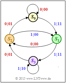
Starting from the adjacent state transition diagram, essential properties and characteristics of the considered rate $1/2$ convolutional code shall be determined, and we explicitly refer to the following theory pages:

In the state transition diagram, the state $S_0$ is always assumed. Two arrows go from each state. The label is "$u_i \hspace{0.05cm}|\hspace{0.05cm} x_i^{(1)}x_i^{(2)}$". For a systematic code, this holds:

The first code bit is identical to the information bit: $\ x_i^{(1)} = u_i ∈ \{0, \, 1\}$
The second code bit is the check bit (parity bit): $\ x_i^{(2)} = p_i ∈ \{0, \, 1\}$.

Hints:

The exercise refers to the chapter "Basics of Turbo Codes".
The following semi–infinite vectors are used in the questions for this exercise:

information sequence $\ \underline{u} = (u_1, \, u_2, \text{ ...})$,
parity sequence $\ \underline{p} = (p_1, \, p_2, \text{ ...})$,
impulse response $\ \underline{g} = (g_1, \, g_2, \text{ ...})$; this is equal to the parity sequence $\underline{p}$ for $\underline{u} = (1, \, 0, \, 0, \text{ ...})$.

Questions

Solution

(1) Correct is the proposed solution 2:

The impulse response $\underline{g}$ is equal to the output sequence $\underline{p}$ for the input sequence $\underline{u} = (1, \, 0, \, 0, \, 0, \text{ ...})$.
Based on the state $S_0$, the state transition diagram results in the following transitions:

$$S_0 → S_1 → S_2 → S_0 → S_0 → S_0 → \text{ ...} \hspace{0.6cm} \Rightarrow \hspace{0.5cm} {\rm impulse\:response} \text{:} \hspace{0.2cm} \underline{g} = (1, \, 0, \, 1, \, 0, \, 0) \, .$$

For a non-recursive filter with memory $m$, $g_i ≡ 0$ holds for $i > m$. In our example, $m = 2$.
In contrast, the proposed solution 1 applies to the recursive filter (RSC) corresponding to "Exercise 4.9".

(2) Let $\underline{u} = (1, \, 0, \, 0, \, 1, \, 0, \, 0, \, u_7)$ and $\underline{g} = (1, \, 0, \, 1, \, 0, \, 0, \, 0, \, ...)$. Then the following holds for the parity sequence due to linearity:

$$\underline{p} \hspace{-0.15cm} \ = \ \hspace{-0.15cm} (\hspace{0.05cm}1,\hspace{0.05cm} 0,\hspace{0.05cm} 0,\hspace{0.05cm} 1,\hspace{0.05cm} 0, \hspace{0.05cm} 0,\hspace{0.05cm} u_7\hspace{0.05cm} ) * (\hspace{0.05cm}1,\hspace{0.05cm} 0,\hspace{0.05cm} 1,\hspace{0.05cm} 0 ,\hspace{0.05cm} 0,\hspace{0.05cm} 0\hspace{0.05cm},\hspace{0.05cm} \text{ ...})= $$

$$\ = \ \hspace{-0.15cm} (\hspace{0.05cm}1,\hspace{0.05cm}\hspace{0.05cm}0,\hspace{0.05cm}1,\hspace{0.05cm}\hspace{0.05cm}0,\hspace{0.05cm} 0,\hspace{0.05cm} 0,\hspace{0.05cm} 0,\hspace{0.05cm} 0,\hspace{0.05cm}0, \hspace{0.05cm} \text{ ...} \hspace{0.05cm})\hspace{0.05cm}\oplus (\hspace{0.05cm}0,\hspace{0.05cm}\hspace{0.05cm}0,\hspace{0.05cm}0,\hspace{0.05cm}\hspace{0.05cm}1,\hspace{0.05cm} 0,\hspace{0.05cm} 1,\hspace{0.05cm} 0,\hspace{0.05cm} 0,\hspace{0.05cm}0, \hspace{0.05cm} \text{ ...}\hspace{0.05cm})\hspace{0.05cm}\oplus (\hspace{0.05cm}0,\hspace{0.05cm}\hspace{0.05cm}0,\hspace{0.05cm}0,\hspace{0.05cm}\hspace{0.05cm}0,\hspace{0.05cm} 0,\hspace{0.05cm} 0,\hspace{0.05cm} u_7,\hspace{0.05cm} 0,\hspace{0.05cm}u_7, \hspace{0.05cm} \text{ ...} \hspace{0.05cm}) $$

$$\Rightarrow \hspace{0.3cm}\underline{p} \hspace{-0.15cm} \ = \ \hspace{-0.15cm} (\hspace{0.05cm}1,\hspace{0.05cm}\hspace{0.05cm}0,\hspace{0.05cm}1,\hspace{0.05cm}\hspace{0.05cm}1,\hspace{0.05cm} 0,\hspace{0.05cm} 1,\hspace{0.05cm} u_7,\hspace{0.05cm} 0,\hspace{0.05cm}u_7, \hspace{0.05cm} \text{ ...} \hspace{0.05cm}) \hspace{0.05cm}.$$

Correct are therefore the proposed solutions 1 and 2 in contrast to the answer 3:

For $u_7 = 1$ gilt $p_7 = 1, \ p_8 = 0, \ p_9 = 1$ and $p_i ≡ 0$ for $i > 9$.

(3) Correct is the proposed solution 2:

From the state transition diagram one can see the code parameters $k = 1$ and $n = 2$.
This means: the transfer function matrix $\mathbf{G}(D)$ consists of two elements ⇒ the proposition 3 is wrong.
The first component of $\mathbf{G}(D)$ is actually 1, since there is a systematic code: $\ \underline{x}^{(1)} ≡ \underline{z}$.
The second component of $\mathbf{G}(D)$ is equal to the $D$–transform of the impulse response $\underline{g}$, where the dummy–variable $D$ indicates a delay of one bit:

$$\underline{g}= (\hspace{0.05cm}1\hspace{0.05cm},\hspace{0.05cm} 0\hspace{0.05cm},\hspace{0.05cm} 1\hspace{0.05cm},\hspace{0.05cm} 0\hspace{0.05cm},\hspace{0.05cm} 0\hspace{0.05cm},\hspace{0.05cm} \text{ ...}\hspace{0.05cm}) \quad \circ\!\!-\!\!\!-^{\hspace{-0.25cm}D}\!\!\!-\!\!\bullet\quad G^{(2)}(D) = 1+ D^2\hspace{0.05cm}. $$

Going beyond the question, we also consider here the filter structure at hand:

Three examples of rate 1/2 convolutional encoders

In the diagram, the encoder considered here is shown as coder $\rm A$ on the left.

This is systematic like the encoder $\rm B$, and
but, unlike coder $\rm B$, is based on a non-recursive filter.
The coder $\rm C$ also has a nonrecursive structure, but is not systematic.
The equivalent systematic representation of encoder $\rm C$ is encoder $\rm B$.

(4) Correct are the proposed solutions 2 and 3:

The exercise could be solved in the same way as subtask (2).
However, we choose here for a change the way about the $D$–transform:

$$\underline{u}= (\hspace{0.05cm}1\hspace{0.05cm},\hspace{0.05cm} 0\hspace{0.05cm},\hspace{0.05cm} 1\hspace{0.05cm},\hspace{0.05cm} 0\hspace{0.05cm},\hspace{0.05cm} 0\hspace{0.05cm},\hspace{0.05cm} 1\hspace{0.05cm}) \quad \circ\!\!-\!\!\!-^{\hspace{-0.25cm}D}\!\!\!-\!\!\bullet\quad U(D) = 1+ D^2 + D^5$$

$$\Rightarrow \hspace{0.3cm} P(D) \hspace{-0.15cm} \ = \ \hspace{-0.15cm} U(D) \cdot G(D) = (1+ D^2 + D^5) \cdot (1+ D^2 ) =1+ D^2 + D^5 + D^2 + D^4 + D^7 = 1+ D^4 + D^5 + D^7$$

$$\Rightarrow \hspace{0.3cm} \underline{p}= (\hspace{0.05cm}1\hspace{0.05cm},\hspace{0.05cm} 0\hspace{0.05cm},\hspace{0.05cm} 0\hspace{0.05cm},\hspace{0.05cm} 0\hspace{0.05cm},\hspace{0.05cm} 1\hspace{0.05cm},\hspace{0.05cm} 1\hspace{0.05cm},\hspace{0.05cm} 0\hspace{0.05cm},\hspace{0.05cm} 1\hspace{0.05cm})\hspace{0.05cm}.$$

(5) Die freie Distanz $d_{\rm F}$ eines Faltungscoders ist gleich der Anzahl der Bits, durch die sich zwei beliebigen Sequenzen dieses Codes mindestens unterscheiden.

Gehen wir wie allgemein üblich als Bezugsgröße von der Nullsequenz $\underline{0} \ \Rightarrow \ S_0 → S_0 → S_0 → S_0 → \ \text{ ...} \ $ aus, so ergibt sich $d_{\rm F}$ gleichzeitig als das minimale Hamming–Gewicht (Anzahl der Einsen) einer zulässigen Codesequenz $\underline{x} ≠ \underline{0}$.

Aus dem Zustandsübergangsdiagramm erkennt man, dass die freie Distanz zum Beispiel durch den Pfad

$$ S_0 → S_0 → S_1 → S_2 → S_0 → S_0 → \text{ ...}$$

gekennzeichnet ist, also durch die Codesequenz $00 \hspace{0.1cm} 11 \hspace{0.1cm} 00 \hspace{0.1cm} 01 \hspace{0.1cm} 00 \text{ ...} \ .$

Dementsprechend gilt für die freie Distanz dieses nichtrekursiven Codes: $\hspace{0.2cm} d_{\rm F} \ \underline{= 3}$.

	$\underline{g} = (1, \, 1, \,1, \, 0, \, 1, \, 1, \, 0, \, 1, \, 1, \text{ ...})$ holds.
	$\underline{g} = (1, \, 0, \, 1, \, 0, \, 0, \, 0, \, 0, \, 0, \, 0, \text{ ...})$ holds.

	The first six bits of the parity sequence are "$1, \, 0, \, 1, \, 1, \, 0, \, 1$".
	With $u_7 = 0$ holds $p_i = 0$ for $i > 6$.
	With $u_7 = 1$ holds $p_i = 0$ for $i > 8$.

	It holds $\mathbf{G}(D) = \big [1, \ 1 + D \big ]$.
	It holds $\mathbf{G}(D) = \big [1, \ 1 + D^2 \big ]$.
	It holds $\mathbf{G}(D) = \big [1 + D^2 \big ]$.

	The first eight bits of the parity sequence are "$1, \, 0, \, 1, \, 1, \, 1, \, 0, \, 1, \, 0$."
	The first eight bits of the parity sequence are "$1, \, 0, \, 0, \, 0, \, 1, \, 1, \, 0, \, 1$".
	It holds $p_i = 0$ for $i ≥ 9$.