Cumulative Distribution Function

Relationship between PDF and CDF

To describe random variables, in addition to the »probability density function» $\rm (PDF)$, we use the »cumulative distribution function« $\rm (CDF)$ which is defined as follows:

$\text{Definition:}$ The »cumulative distribution function« $F_{x}(r)$ corresponds to the probability that the random variable $x$ is less than or equal to a real number $r$:

$$F_{x}(r) = {\rm Pr}( x \le r).$$

For a value-continuous random variable, the following statements are possible regarding the CDF:

The CDF is computable from the probability density function $f_{x}(x)$ by integration. It holds:

$$F_{x}(r) = \int_{-\infty}^{r}f_x(x)\,{\rm d}x.$$

Since the PDF is never negative, $F_{x}(r)$ increases at least weakly monotonically, and the function always lies between the following limits:

$$F_{x}(r → \hspace{0.05cm} - \hspace{0.05cm} ∞) = 0, \hspace{0.5cm}F_{x}(r → +∞) = 1.$$

Inversely, the probability density function can be determined from the CDF by differentiation:

$$f_{x}(x)=\frac{{\rm d} F_{x}(r)}{{\rm d} r}\Bigg |_{\hspace{0.1cm}r=x}.$$

The addition »$r = x$« makes it clear that in our nomenclature the PDF argument is the random variable $x$ itself, while the CDF argument specifies any real variable $r$ .

$\text{Notes on nomenclature:}$ If in the definitions of $\rm PDF$ and $\rm CDF$ we had distinguished

between the random variable $X$

and the realizations $x ∈ X$ ⇒ $f_{X}(x), F_{X}(x)$,

we would have the following nomenclature:

$$F_{X}(x) = {\rm Pr}(X \le x) = \int_{-\infty}^{x}f_{x}(\xi)\,{\rm d}\xi.$$

Unfortunately, at the beginning of our $\rm LNTwww$ project $(2001)$ we decided to use our nomenclature for quite legitimate reasons, which now $(2017)$ cannot be changed, also with regard to the realized learning videos. So we stick with $f_{x}(x)$ instead of $f_{X}(x)$ as well as $F_{x}(r)$ instead of $F_{X}(x).$

CDF for value-continuous random variables

The equations given in the last section apply only to value-continuous random variables and will be illustrated here by an example. In the next section it will be shown that for »value-discrete random variables« the equations must be modified somewhat.

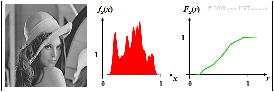
$\text{Example 1:}$ The left image shows the photo »Lena«, which is often used as a test template for image coding procedures.

PDF and CDF of a value-continuous image

If this image is divided into $256 × 256$ pixels, and the brightness is determined for each pixel, a sequence $〈x_ν〉$ of gray values is obtained whose length $N = 256^2 = 65\hspace{0.06cm}536$.

The gray value $x$ is a value-continuous random variable, where the assignment to numerical values is arbitrary. For example, let »black« be characterized by $x = 0$ and »white« by $x = 1$: The value $x =0.5$ then characterizes a medium gray coloration.

The middle diagram shows the PDF $f_{x}(x)$ which is also often referred to in the literature as »gray value statistics«.

In the original image some gray values are preferred and the two extreme values $x =0$ ("deep black") or $x =1$ ("pure white") occur very rarely.

The cumulative distribution function $F_{x}(r)$ is continuous in value and increases monotonically from $0$ to $1$ as the right figure shows.

For $r \approx 0$ and $r \approx 1$ the CDF is horizontal due to the lack of PDF components.

$\text{Note:}$ Strictly speaking, for an image that can be displayed on a computer $($in contrast to an analog photograph$)$:

The gray value is always a discrete in value.
However, with large resolution of the color information $($»color depth«$)$, this random variable can be approximated to be continuous in value.

» The topic of this chapter is illustrated with examples in the (German language) learning video
»Zusammenhang zwischen WDF und VTF» $\Rightarrow$ »Relationship between PDF and CDF«.

CDF for value-discrete random variables

For the CDF calculation of a value-discrete random variable $x$ from its PDF, a more general equation must always be assumed. Here, with the auxiliary variable $\varepsilon > 0$:

$$F_{x}(r)=\lim_{\varepsilon\hspace{0.05cm}\to \hspace{0.05cm}0}\int_{-\infty}^{r+\varepsilon}f_x(x)\,{\rm d}x.$$

Due to the »less than/equal» sign in the »general definition«, a limit value must be formed for the CDF calculation. If we also take into account that, for a value-discrete random variable, the PDF consists of a sum of weighted »Dirac delta functions«, we obtain:

$$F_{x}(r)=\lim_{\varepsilon\hspace{0.05cm}\to \hspace{0.05cm} 0}\int_{-\infty}^{r+\varepsilon}\sum\limits_{\mu= 1}^{ M}p_\mu\cdot \delta(x-x_\mu)\,{\rm d}x.$$

If we interchange integration and summation in this equation, and consider that an integration over the Dirac delta function yields the step function, we obtain:

$$F_{x}(r)=\sum\limits_{\mu= \rm 1}^{\it M}p_\mu\cdot \gamma_0 (r-x_\mu),\hspace{0.4cm}{\rm with} \hspace{0.4cm}\gamma_0(x)=\lim_{\epsilon\hspace{0.05cm}\to \hspace{0.05cm} 0}\int_{-\infty}^{x+\varepsilon}\delta (u)\,{\rm d} u = \left\{ \begin{array}{*{2}{c}} 0 \hspace{0.4cm} {\rm if}\hspace{0.1cm} x< 0,\\ 1 \hspace{0.4cm} {\rm if}\hspace{0.1cm}x\ge 0. \\ \end{array} \right.$$

The function $γ_0(x)$ differs from the »unit step function« $γ(x)$ often used in systems theory in that at the jump point $x = 0$ the right-hand side limit $1$nbsp; is valid $($instead of the mean value $0.5$ between left– and right–hand side limits$)$.

With the above CDF definition, the following probability equation holds for value-continuous and value-discrete random variables equally, and of course also for mixed random variables with discrete and continuous parts:

$${\rm Pr}(x_{\rm u}<x \le x_{\rm o})=F_x(x_{\rm o})-F_x(x_{\rm u}).$$

For purely value-continuous random variables, the »less than« sign and the »less than/equal to« sign could be substituted for each other here.

$${\rm Pr}(x_{\rm u}<x \le x_{\rm o}) ={\rm Pr}(x_{\rm u}\le x \le x_{\rm o}) ={\rm Pr}(x_{\rm u}\le x < x_{\rm o}) ={\rm Pr}(x_{\rm u}<x < x_{\rm o}).$$

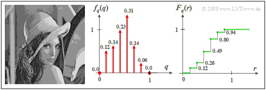
$\text{Example 2:}$ If the gray value of the »original Lena photo« is quantized by eight levels, so that each pixel can be represented by three bits and transmitted digitally, the discrete random variable $q$ is obtained. However, due to the quantization, a part of the image information is lost, which is reflected in the quantized image by clearly recognizable »contours«.

PDF and CDF of a value-discrete image

The associated PDF $f_{q}(q)$ is composed of $M = 8$ Dirac delta functions, where, in the quantization chosen here, the possible gray levels are assigned the values $q_\mu = (\mu - 1)/7$ with $\mu = 1, 2,$ ... , $8$.

The weights of the Dirac delta functions can be calculated from the PDF $f_{x}(x)$ of the original image. One obtains

$$p_\mu={\rm Pr}(q = q_\mu ) = {\rm Pr}(\frac{2\mu-\rm 3}{14}< {x} \le\frac{2\it \mu- \rm 1}{14}) $$

$$\Rightarrow \hspace{0.3cm} p_\mu={\rm Pr}(q = q_\mu ) = \int_{(2\it \mu- \rm 3)/14}^{(2\mu-1)/14}\it f_{x}{\rm (}x{\rm )}\,{\rm d}x.$$

For the undefined areas $(x<0$, $x>1)$ is to be set $f_{x}(x) = 0$. Since in the original image the gray levels $x ≈0$ $($»very deep black«$)$ or $x ≈1$ $($»almost pure white«$)$ are largely missing, $p_1 ≈ p_8 ≈ 0$ result.

Thus, only six Dirac delta functions are visible in the PDF. The two missing Diracs at $q = 0$ and $q =1$ are only indicated by dots.

The step-shaped CDF $F_{q}(r)$ sketched on the right thus has six points of discontinuity, where in each case the right-hand side limit is valid.

.

» The topic of this chapter is illustrated with examples in the (German language) learning video
»Zusammenhang zwischen WDF und VTF» $\Rightarrow$ »Relationship between PDF and CDF«.

Exercises for the chapter

Exercise 3.2: CDF for Exercise 3.1

Exercise 3.2Z: Relationship between PDF and CDF

Cumulative Distribution Function

Contents

Relationship between PDF and CDF

CDF for value-continuous random variables

CDF for value-discrete random variables

Exercises for the chapter