Exercise 1.3: Rayleigh Fading
From LNTwww
Rayleigh–Fading should be used when
- there is no direct connection between sender and receiver, and
- the signal reaches the receiver in many ways, but their transit times are approximately the same.
An example of such a Rayleigh–channel occurs in urban mobile communications when narrowband signals are used with ranges between $50$ and $100$ meters.
Looking at the radio signals $s(t)$ and $r(t)$ in the equivalent low-pass range $($that is, around the frequency $f = 0)$, the signal transmission is given by the equation
- $$r(t)= z(t) \cdot s(t)$ described completely. The multiplicative falsification :$$z(t)= x(t) + {\rm j} \cdot y(t)$$ is always complex and has the following characteristics: * The real part $x(t)$ and the imaginary part $y(t)$ are Gaussian mean-free random variables, both with equal variance $\sigma^2$. Within the components $x(t)$ and $y(t)$ there may be statistical bindings, but this is not relevant for the solution of the present task. There are no bonds between $x(t)$ and $y(t)$; their cross-correlation function is identical to zero. * The amount $a(t) = |z(t)|$ has a Rayleigh–WDF, from which the name „<i>Rayleigh–Fading</i>” is derived: :$$f_a(a) =
\left\{ \begin{array}{c} a/\sigma^2 \cdot {\rm e}^ { -a^2/(2\sigma^2)} \\\ 0 \end{array} \right.\quad \begin{array}{*{*{1}c} {\rm f\ddot{u}r}\hspace{0.15cm} a \ge 0 \\ {\rm f\ddot{u}r}\hspace{0.15cm} a < 0 \\\ \\ \end{array}
\hspace{0.05cm}.$$

* The absolute square  $p(t) = a(t)^2 = |z(t)|^2$  is exponentially distributed according to the equation
$$f_p(p) = \left\{ \begin{array}{c} 1/(2\sigma^2) \cdot {\rm e}^ { -p/(2\sigma^2)} \\
0 \end{array} \right.\quad
\begin{array}{*{*{1}c} {\rm f\ddot{u}r}\hspace{0.15cm} p \ge 0 \\ {\rm f\ddot{u}r}\hspace{0.15cm} p < 0 \\\ \\ \end{array}
\hspace{0.05cm}.$$

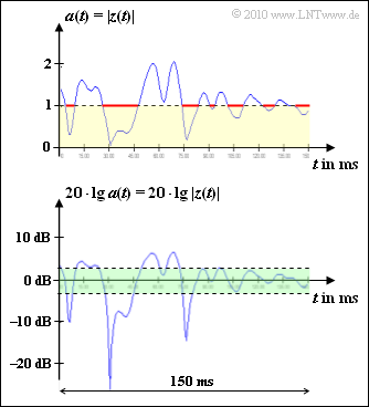
Measurements have shown that the time intervals with  $a(t) ≤ 1$  (highlighted in yellow in the graphic) add up to  $\text{59 ms}$  (areas highlighted in red). With the total measurement time of  $\text{150 ms}$  the probability that the amount of the <i>Rayleigh–fading</i> is less than or equal to  $1$  results in
$${\rm Pr}(a(t) \le 1) = \frac{59\,\,{\,{\rm ms}}}{150\,\,{\rm ms}} = 39.4 \%
\hspace{0.05cm}.$$

In the lower graphic the value range between  $\text{-3 dB}$  and  $\text{+3 dB}$  regarding the logarithmic Rayleigh–Size  $20 \cdot {\rm lg} is highlighted in green. \ a(t)$. The subtask '''(4)'' refers to this.


''Notes:''
* The task belongs to chapter  [[Mobile_Communications/Probability Density_of_Rayleigh%E2%80%93Fadings|Probability Density of Rayleigh–Fadings]]  of this book.
* A similar topic is treated with a different approach in chapter  [[Stochastic_Signal Theory/Weitere_Verteilungen|Weitere Verteilungen]]  of the book „Stochastic Signal Theory”.
* To check your results you can use the interactive applet  [[Applets:WDF_VTF|WDF, VTF and Moments]]  of the book „Stochastic Signal Theory”.


==='"`UNIQ--h-0--QINU`"'Questionnaire===

'"`UNIQ--quiz-00000002-QINU`"'

==='"`UNIQ--h-1--QINU`"'Sample solution===
'"`UNIQ--html-00000003-QINU`"'
'''(1)''  From ${\rm Max}[a(t)] = 2$ follows directly:
$${\rm Max} \left [ 20 \cdot {\rm lg}\hspace{0.15cm}a(t) \right ] = 20 \cdot {\rm lg}\hspace{0.15cm}(2) \hspace{0.15cm} \underline{\approx 6\,\,{\rm dB}}
 \hspace{0.05cm}.$$


'''(2)'''  The maximum value of the square $p(t) = a(t)^2$ is
$$${\rm Max} \left [ p(t) \right ] = {\rm Max} \left [ a(t)^2 \right ] \hspace{0.15cm} \underline{\4}
  \hspace{0.05cm}.'"`UNIQ-MathJax22-QINU`"'10 \cdot {\rm lg}\hspace{0.15cm} p(t) = 10 \cdot {\rm lg}\hspace{0.15cm}a(t)^2 = 20 \cdot {\rm lg}\hspace{0.15cm} a(t)
  \hspace{0.05cm}.'"`UNIQ-MathJax23-QINU`"'f_p(p) = \frac{1}{2\sigma^2} \cdot {\rm exp} [ -\frac{p}{2\sigma^2}]
 \hspace{0.05cm}.'"`UNIQ-MathJax24-QINU`"'{\rm Pr}(p(t) \le 1) = \frac{1}{2\sigma^2} \cdot \int_{0}^{1}{\rm exp} [ -\frac{p}{2\sigma^2}] \hspace{0.15cm}{\rm d}p =
 1 - {\rm exp} [ -\frac{1}{2\sigma^2}] = 0.394'"`UNIQ-MathJax25-QINU`"'\Rightarrow \hspace{0.3cm} {\rm exp} [ -\frac{1}{2\sigma^2}] = 0.606 \hspace{0.3cm} \Rightarrow \hspace{0.3cm}
 \sigma^2 = \frac{1}{2 \cdot {\rm ln}\hspace{0.1cm}(0.606)} = 1 \hspace{0.3cm} \Rightarrow \hspace{0.3cm}
 \underline{\sigma = 1} \hspace{0.05cm}.'"`UNIQ-MathJax26-QINU`"'{\rm Pr}(-3\,\,{\rm dB}\le 10 \cdot {\rm lg}\hspace{0.15cm}p(t) \le +3\,\,{\rm dB}) \hspace{-0.1cm} \ = \ \hspace{-0.1cm}   \int_{0.5}^{2}f_p(p)\hspace{0.15cm}{\rm d}p =
  \left [ - {\rm e}^{ -{p}/(2\sigma^2)}\hspace{0.15cm} \right ]_{0.5}^{2} ={\rm e}^{-0.25}- {\rm e}^{-1} \approx 0.779 - 0.368 \hspace{0.15cm} \underline{ = 0.411} \hspace{0.05cm}.$$
