Difference between revisions of "Aufgaben:Exercise 1.5: Rectangular-in-Frequency Low-Pass Filter"
| (54 intermediate revisions by 4 users not shown) | |||
| Line 1: | Line 1: | ||
| − | {{quiz-Header|Buchseite= | + | {{quiz-Header|Buchseite=Linear_and_Time_Invariant_Systems/Some_Low-Pass_Functions_in_Systems_Theory}} |
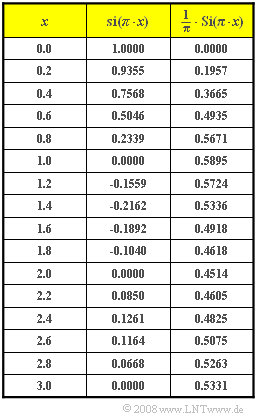
| − | [[File:P_ID852__LZI_A_1_5.png|right| | + | [[File:P_ID852__LZI_A_1_5.png|right|frame|Table with values of the $\rm si$–function and the $\rm Si$–function]] |
| − | + | We consider an ideal, rectangular low-pass filter – also called a Küpfmüller low-pass filter, | |
| − | * | + | *which passes all frequencies $f < 5 \ \rm kHz$ in an undistorted way ⇒ $H(f) = 1$, |
| − | * | + | *and completely suppresses all spectral components above $5 \ \rm kHz$ ⇒ $H(f) = 0$. |
| − | + | Exactly at the cut-off frequency $f_{\rm G} = 5 \ \rm kHz$ the value of the transfer function is equal to $1/2$. | |
| − | + | Various signals are applied to the input of the low-pass filter: | |
| − | * | + | *a narrow rectangular pulse of suitable height which can be approximated by a "Dirac": |
| − | $$x_1(t) = 10^{-3}\hspace{0.1cm}{\rm Vs} \cdot {\rm \delta}(t),$$ | + | :$$x_1(t) = 10^{-3}\hspace{0.1cm}{\rm Vs} \cdot {\rm \delta}(t),$$ |
| − | * | + | *a Dirac pulse, i.e., a sum of Dirac functions evaluated at the respective time interval of $T_{\rm A}$: |
| − | $$x_2(t) = 10^{-3}\hspace{0.1cm}{\rm Vs} \cdot \sum_{\nu = -\infty}^{+\infty}{\rm \delta}(t - \nu \cdot T_{\rm A}),$$ | + | :$$x_2(t) = 10^{-3}\hspace{0.1cm}{\rm Vs} \cdot \sum_{\nu = -\infty}^{+\infty}{\rm \delta}(t - \nu \cdot T_{\rm A}),$$ |
| − | : | + | :where the associated spectrum with $f_{\rm A} = 1/T_{\rm A}$ is: |
| − | $$X_2(f) = \frac{10^{-3}\hspace{0.1cm}{\rm Vs}}{T_{\rm A}} \cdot\sum_{\mu = -\infty}^{+\infty}{\rm \delta}(f - \mu \cdot f_{\rm A}),$$ | + | :$$X_2(f) = \frac{10^{-3}\hspace{0.1cm}{\rm Vs}}{T_{\rm A}} \cdot\sum_{\mu = -\infty}^{+\infty}{\rm \delta}(f - \mu \cdot f_{\rm A}),$$ |
| − | * | + | *a step function at time $t = 0$: |
| − | $$x_3(t) = 10\hspace{0.1cm}{\rm V} \cdot \gamma(t) = \left\{ \begin{array}{c} 0 \\ 5\hspace{0.1cm}{\rm V} \\ 10\hspace{0.1cm}{\rm V} \\ \end{array} \right.\quad \quad\begin{array}{*{10}c} {\rm{f\ddot{u}r}} \\ {\rm{f\ddot{u}r}}\\ {\rm{f\ddot{u}r}} \\ \end{array}\begin{array}{*{20}c}{ t < 0,} \\{ t = 0,} \\ | + | :$$x_3(t) = 10\hspace{0.1cm}{\rm V} \cdot \gamma(t) = \left\{ \begin{array}{c} 0 \\ 5\hspace{0.1cm}{\rm V} \\ 10\hspace{0.1cm}{\rm V} \\ \end{array} \right.\quad \quad\begin{array}{*{10}c} {\rm{f\ddot{u}r}} \\ {\rm{f\ddot{u}r}}\\ {\rm{f\ddot{u}r}} \\ \end{array}\begin{array}{*{20}c}{ t < 0,} \\{ t = 0,} \\ |
{ t > 0,} \\ \end{array}$$ | { t > 0,} \\ \end{array}$$ | ||
| − | * | + | *an $\rm si$–shaped pulse with equivalent duration $T$: |
| − | $$x_4(t) = 10\hspace{0.1cm}{\rm V} \cdot {\rm si}(\pi \cdot {t}/{T}) .$$ | + | :$$x_4(t) = 10\hspace{0.1cm}{\rm V} \cdot {\rm si}(\pi \cdot {t}/{T}) \hspace{0.5cm} {\rm mit} \hspace{0.5cm} {\rm si}(x) = {\rm sin}(x)/x .$$ |
| − | |||
| − | |||
| − | === | + | |
| + | |||
| + | |||
| + | |||
| + | |||
| + | ''Please note:'' | ||
| + | *The exercise belongs to the chapter [[Linear_and_Time_Invariant_Systems/Some_Low-Pass_Functions_in_Systems_Theory|Some Low-Pass Functions in Systems Theory]]. | ||
| + | *The table lists the function values of the ''sinc function'' ${\rm si}(πx)$ and the ''sine integral function'' ${\rm Si}(πx)$: | ||
| + | :$${\rm Si}(\pi x) = \int_{ 0 }^{ x } {{\rm si} ( \pi \xi )} \hspace{0.1cm}{\rm d}\xi \hspace{0.5cm}{\rm mit } \hspace{0.5cm} {\rm si}(x) =\sin(x)/x.$$ | ||
| + | |||
| + | |||
| + | |||
| + | |||
| + | |||
| + | ===Questions=== | ||
<quiz display=simple> | <quiz display=simple> | ||
| − | { | + | {What is the output signal $y_1(t)$ in response to the Dirac function $x_1(t)$, in particular at times $t = 0$ and $t = 50 \ \rm µ s$? |
|type="{}"} | |type="{}"} | ||
| − | $y_1(t = 0) =$ { 10 } V | + | $y_1(t = 0) \ = \ $ { 10 3% } $\rm V$ |
| − | $y_1(t = 50 {\: \rm | + | $y_1(t = 50 {\: \rm µ s}) \ = \ $ { 6.37 3% } $\rm V$ |
| − | { | + | {What is the output signal $y_2(t)$, if the dirac pulse $x_2(t)$ is applied to the filter input and $T_{\rm A} = 200 \ µ \rm s$ holds. What signal value occurs at $t = 0$ ? |
|type="{}"} | |type="{}"} | ||
| − | $ | + | $y_2(t = 0) \ = \ $ { 10 3% } $\rm V$ |
| − | { | + | {What values $y_2(t = 0)$ are obtained with $T_{\rm A} = 199 \ \rm µ s$ or $T_{\rm A} = 201 \ \rm µ s$? |
|type="{}"} | |type="{}"} | ||
| − | $T_{\rm A} = {\rm | + | $T_{\rm A} = 199 \ {\rm µ s} \text{:}\hspace{0.4cm} y_2(t = 0) \ = \ $ { 5.025 3% } $\rm V$ |
| − | $T_{\rm A} = {\rm | + | $T_{\rm A} = 201 \ {\rm µ s} \text{:}\hspace{0.4cm} y_2(t = 0) \ = \ $ { 14.925 3% } $\rm V$ |
| − | { | + | {State the output signal $y_3(t)$ for the step function $x_3(t)$ with final value $10 \ \rm V$ . What is the signal value at time $t = 0$ ? |
|type="{}"} | |type="{}"} | ||
| − | $y_3(t = 0) =$ { 5 } V | + | $y_3(t = 0) \ = \ $ { 5 3% } $\rm V$ |
| − | { | + | {At what time $t_{\rm max}$ does $y_3(t)$ attain its maximum value? What is the maximum value?? |
|type="{}"} | |type="{}"} | ||
| − | $t_{\rm max} =$ { 100 } $\rm | + | $t_{\rm max} \ = \ $ { 100 3% } $\rm µ s$ |
| − | $y_3(t_{\rm max}) =$ { 10.895 | + | $y_3(t_{\rm max}) \ = \ $ { 10.895 3% } $\rm V$ |
| − | { | + | {What is the output signal $y_4(t)$, if the ${\rm si}$–shaped signal $x_4(t)$ with ${\rm si}(πx)$ $T = 200 \ \rm µ s$ is applied to the input? What value is obtained for $t = 0$? |
|type="{}"} | |type="{}"} | ||
| − | $ | + | $y_4(t = 0) \ = \ $ { 10 3% } $\rm V$ |
| − | { | + | {What signal value $y_4(t = 0)$ is obtained for $T = 50 \ \rm µ s$? |
|type="{}"} | |type="{}"} | ||
| − | $ | + | $y_4(t = 0) \ = \ $ { 5 3% } $\rm V$ |
</quiz> | </quiz> | ||
| − | === | + | ===Solution=== |
{{ML-Kopf}} | {{ML-Kopf}} | ||
| − | ''' | + | '''(1)''' With $Δf = 10 \ \rm kHz$, the impulse response of the ideal low-pass filter is given by: |
| − | $$h(t) = \Delta f \cdot {\rm si}(\pi \cdot \Delta f \cdot t ).$$ | + | :$$h(t) = \Delta f \cdot {\rm si}(\pi \cdot \Delta f \cdot t ).$$ |
| − | + | *The output signal differs from this by the weighting factor $\rm 10^{–3} \ \rm Vs$: | |
| − | $$ | + | :$$y_1(t) = 10^{-3}\hspace{0.1cm}{\rm Vs} \cdot 10^{4}\hspace{0.1cm}{\rm Hz} \cdot {\rm si}(\pi \cdot \Delta f \cdot t ) = 10\hspace{0.1cm}{\rm V} \cdot {\rm si}(\pi \cdot \Delta f \cdot t )$$ |
| − | si} \left( | + | :$$ \Rightarrow \hspace{0.2cm}y_1(t = 0) \hspace{0.15cm}\underline{=10\hspace{0.1cm}{\rm V}},\hspace{0.5cm}y_1(t = 50\hspace{0.1cm}{\rm µ s}) =10\hspace{0.1cm}{\rm V} \cdot {\rm |
| + | si} \left( {\pi}/{2} \right) \hspace{0.15cm}\underline{= 6.37\hspace{0.1cm}{\rm V}}.$$ | ||
| + | |||
| + | |||
| + | |||
| + | [[File:EN_LZI_A_1_5_b.png | rechts |frame| Dirac pulse and rectangular filter]] | ||
| + | '''(2)''' The spectrum $X_2(f)$ contains discrete lines at an interval of $f_{\rm A} = 1/T_{\rm A} = 5 \ \rm kHz$, each with weight $5 \ \rm V$. | ||
| + | |||
| + | *The spectrum $Y_2(f)$ thus consists of one spectral line at $f = 0$ with weight $5 \ \rm V$ and one each at $±5 \ \rm kHz$ with weight $2.5 \ \rm V$. Hence, the following is true for the time signal: | ||
| + | :$$ y_2(t) = 5 \hspace{0.1cm}{\rm V} + 5\hspace{0.1cm}{\rm V} \cdot{\rm cos}(2 \pi \cdot f_{\rm A} \cdot t ) = 10\hspace{0.1cm}{\rm V} \cdot {\rm cos}^2(\pi \cdot f_{\rm A} \cdot t ).$$ | ||
| + | :$$ \Rightarrow \hspace{0.3cm} y_2(t= 0) \hspace{0.15cm} \underline{ = 10\hspace{0.1cm}{\rm V}} .$$ | ||
| − | |||
| − | |||
| − | |||
| − | ''' | + | '''(3)''' Due to $T_{\rm A} = 199 \ \rm µ s $ , $f_{\rm A} > 5 \ \rm kHz$ holds. Because of $H(f_{\rm A}) = 0$ the spectrum consists of only one spectral line at $f = 0$ with weight $5.025 \ \rm V$ and the following constant curve is obtained |
| + | :$$ \Rightarrow \hspace{0.3cm} y_2(t) \rm \underline{\: = 5.025 \ \rm V}.$$ | ||
| + | |||
| + | *If $T_{\rm A}$ is further decreased, the output still yields a direct signal but with larger signal value (proportional to $1/T_{\rm A}$). | ||
| − | + | *In contrast to this, with $T_{\rm A} = 201 \ \rm µ s $ the sampling frequency is slightly smaller than the cut-off frequency of the filter $(5 \ \rm kHz)$ and the spectral function of the output signal is: | |
| − | $$Y_2(f) = 4.975\hspace{0.1cm}{\rm V} \cdot \ | + | :$$Y_2(f) = 4.975\hspace{0.1cm}{\rm V} \cdot \big[ {\rm \delta}(f ) + {\rm \delta}(f + f_{\rm A}) + {\rm \delta}(f - f_{\rm A})\big].$$ |
| − | + | *From this it follows for the time signal: | |
| − | $$y_2(t ) = 4.975\hspace{0.1cm}{\rm V} + 9.95\hspace{0.1cm}{\rm | + | :$$y_2(t ) = 4.975\hspace{0.1cm}{\rm V} + 9.95\hspace{0.1cm}{\rm |
V} \cdot {\rm cos}(2 \pi \cdot f_{\rm A} \cdot t ) \hspace{0.2cm} \Rightarrow | V} \cdot {\rm cos}(2 \pi \cdot f_{\rm A} \cdot t ) \hspace{0.2cm} \Rightarrow | ||
\hspace{0.2cm}y_2(t = 0) \hspace{0.15cm}\underline{=14.925\hspace{0.1cm}{\rm V}}.$$ | \hspace{0.2cm}y_2(t = 0) \hspace{0.15cm}\underline{=14.925\hspace{0.1cm}{\rm V}}.$$ | ||
| − | + | *Nothing changes in the fundamental curve as long as $ 200 \ {\rm µ s} < T_{\rm A} < 400 \ {\rm µ s} $ holds. | |
| + | *However, different amplitudes arise as a result depending on $T_{\rm A}$ . For $T_{\rm A} ≥ 400 \ {\rm µ s}$ additional spectral lines are added. | ||
| + | |||
| + | |||
| + | |||
| + | [[File:P_ID854__LZI_A_1_5_d.png | rechts |frame| Impulse response and step response]] | ||
| + | '''(4)''' The output signal $y_3(t)$ now goes according to the sine integral function: | ||
| + | :$$y_3(t = 0) = 10\hspace{0.1cm}{\rm V} \cdot \Delta f \cdot \int_{ - \infty }^{ t } \hspace{-0.3cm} {{\rm si} ( \pi \Delta f \tau )} \hspace{0.1cm}{\rm d}\tau = 10\hspace{0.1cm}{\rm V} \cdot \big[ {1}/{2} + {1}/{\pi}\cdot {\rm Si} ( \pi \Delta f t )\big].$$ | ||
| + | :$$ \Rightarrow \hspace{0.3cm} y_3(t= 0) \hspace{0.15cm} \underline{ = 5\hspace{0.1cm}{\rm V}} .$$ | ||
| + | |||
| + | |||
| + | '''(5)''' It is obvious that $y_3(t)$ attains its maximum when the ${\rm si}$–function intersects the abscissa for the first time at positive times (see sketch). So, it must hold:: | ||
| + | :$$t_{\rm max} = 1/Δf \rm \underline{\: = 100 \: µ s}.$$ | ||
| − | + | *The signal value is obtained according to the table on the information page and is | |
| − | + | :$$y_3(t = t_{\rm max}) = 10\hspace{0.1cm}{\rm V} \cdot \big[ {1}/{2} + {1}/{\pi}\cdot | |
| − | + | {\rm Si} ( \pi )\big]= 10\hspace{0.1cm}{\rm V} \cdot \big[ 0.5 + | |
| + | 0.5895 \big] \hspace{0.15cm}\underline{= 10.895 \hspace{0.1cm}{\rm V}} .$$ | ||
| + | *At later times $t$ , $y_3(t)$ slowly adjusts to its final value $10 \ \rm V$. | ||
| − | ''' | + | [[File:P_ID855__LZI_A_1_5_f.png | rechts |frame|Rectangular spectra at the input of the rectangular filter]] |
| − | $$ | + | '''(6)''' The spectral function $X_4(f)$ is rectangular like $H(f)$ and for $|f| > 2.5 \ \rm kHz$ always zero. |
| − | + | *This means that $Y_4(f ) = X_4(f)$ holds and so does $y_4(t) = x_4(t)$. | |
| − | + | *Thus, $y_4(t = 0) \rm \underline{\: = 10 \: \rm V}$. | |
| − | |||
| − | |||
| + | '''(7)''' Due to $T = 50 \ \rm µ s$ , $X_4(f)$ has the width $20 \ \rm kHz$ and the height $0.5 · 10 ^{-3} \ \rm V/Hz$. | ||
| − | + | *The spectral function $Y_4(f)$ has the same height after being multiplied by $H(f)$ . | |
| − | $$ | + | *The width $10 \ \rm kHz$ is now determined exclusively by $H(f)$ : |
| − | Hz} } \cdot 10 \hspace{0.1cm}{\rm kHz} \cdot {\rm si}(\pi \Delta f t ) = 5\hspace{0.1cm}{\rm V} \cdot {\rm si}(\pi \Delta f t ) | + | :$$y_4(t) = 0.5 \cdot 10^{-3}\hspace{0.1cm}{ {\rm V} }/{ {\rm |
| + | Hz} } \cdot 10 \hspace{0.1cm}{\rm kHz} \cdot {\rm si}(\pi \Delta f t ) = 5\hspace{0.1cm}{\rm V} \cdot {\rm si}(\pi \Delta f t )$$ | ||
| + | :$$ \Rightarrow \hspace{0.3cm}y_4(t = 0) \hspace{0.15cm}\underline{=5\hspace{0.1cm}{\rm V} }.$$ | ||
{{ML-Fuß}} | {{ML-Fuß}} | ||
| − | [[Category: | + | [[Category:Linear and Time-Invariant Systems: Exercises|^1.3 Some Low-Pass Functions in Systems Theory^]] |
Latest revision as of 15:35, 7 October 2021
We consider an ideal, rectangular low-pass filter – also called a Küpfmüller low-pass filter,
- which passes all frequencies $f < 5 \ \rm kHz$ in an undistorted way ⇒ $H(f) = 1$,
- and completely suppresses all spectral components above $5 \ \rm kHz$ ⇒ $H(f) = 0$.
Exactly at the cut-off frequency $f_{\rm G} = 5 \ \rm kHz$ the value of the transfer function is equal to $1/2$.
Various signals are applied to the input of the low-pass filter:
- a narrow rectangular pulse of suitable height which can be approximated by a "Dirac":
- $$x_1(t) = 10^{-3}\hspace{0.1cm}{\rm Vs} \cdot {\rm \delta}(t),$$
- a Dirac pulse, i.e., a sum of Dirac functions evaluated at the respective time interval of $T_{\rm A}$:
- $$x_2(t) = 10^{-3}\hspace{0.1cm}{\rm Vs} \cdot \sum_{\nu = -\infty}^{+\infty}{\rm \delta}(t - \nu \cdot T_{\rm A}),$$
- where the associated spectrum with $f_{\rm A} = 1/T_{\rm A}$ is:
- $$X_2(f) = \frac{10^{-3}\hspace{0.1cm}{\rm Vs}}{T_{\rm A}} \cdot\sum_{\mu = -\infty}^{+\infty}{\rm \delta}(f - \mu \cdot f_{\rm A}),$$
- a step function at time $t = 0$:
- $$x_3(t) = 10\hspace{0.1cm}{\rm V} \cdot \gamma(t) = \left\{ \begin{array}{c} 0 \\ 5\hspace{0.1cm}{\rm V} \\ 10\hspace{0.1cm}{\rm V} \\ \end{array} \right.\quad \quad\begin{array}{*{10}c} {\rm{f\ddot{u}r}} \\ {\rm{f\ddot{u}r}}\\ {\rm{f\ddot{u}r}} \\ \end{array}\begin{array}{*{20}c}{ t < 0,} \\{ t = 0,} \\ { t > 0,} \\ \end{array}$$
- an $\rm si$–shaped pulse with equivalent duration $T$:
- $$x_4(t) = 10\hspace{0.1cm}{\rm V} \cdot {\rm si}(\pi \cdot {t}/{T}) \hspace{0.5cm} {\rm mit} \hspace{0.5cm} {\rm si}(x) = {\rm sin}(x)/x .$$
Please note:
- The exercise belongs to the chapter Some Low-Pass Functions in Systems Theory.
- The table lists the function values of the sinc function ${\rm si}(πx)$ and the sine integral function ${\rm Si}(πx)$:
- $${\rm Si}(\pi x) = \int_{ 0 }^{ x } {{\rm si} ( \pi \xi )} \hspace{0.1cm}{\rm d}\xi \hspace{0.5cm}{\rm mit } \hspace{0.5cm} {\rm si}(x) =\sin(x)/x.$$
Questions
Solution
- $$h(t) = \Delta f \cdot {\rm si}(\pi \cdot \Delta f \cdot t ).$$
- The output signal differs from this by the weighting factor $\rm 10^{–3} \ \rm Vs$:
- $$y_1(t) = 10^{-3}\hspace{0.1cm}{\rm Vs} \cdot 10^{4}\hspace{0.1cm}{\rm Hz} \cdot {\rm si}(\pi \cdot \Delta f \cdot t ) = 10\hspace{0.1cm}{\rm V} \cdot {\rm si}(\pi \cdot \Delta f \cdot t )$$
- $$ \Rightarrow \hspace{0.2cm}y_1(t = 0) \hspace{0.15cm}\underline{=10\hspace{0.1cm}{\rm V}},\hspace{0.5cm}y_1(t = 50\hspace{0.1cm}{\rm µ s}) =10\hspace{0.1cm}{\rm V} \cdot {\rm si} \left( {\pi}/{2} \right) \hspace{0.15cm}\underline{= 6.37\hspace{0.1cm}{\rm V}}.$$
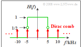
(2) The spectrum $X_2(f)$ contains discrete lines at an interval of $f_{\rm A} = 1/T_{\rm A} = 5 \ \rm kHz$, each with weight $5 \ \rm V$.
- The spectrum $Y_2(f)$ thus consists of one spectral line at $f = 0$ with weight $5 \ \rm V$ and one each at $±5 \ \rm kHz$ with weight $2.5 \ \rm V$. Hence, the following is true for the time signal:
- $$ y_2(t) = 5 \hspace{0.1cm}{\rm V} + 5\hspace{0.1cm}{\rm V} \cdot{\rm cos}(2 \pi \cdot f_{\rm A} \cdot t ) = 10\hspace{0.1cm}{\rm V} \cdot {\rm cos}^2(\pi \cdot f_{\rm A} \cdot t ).$$
- $$ \Rightarrow \hspace{0.3cm} y_2(t= 0) \hspace{0.15cm} \underline{ = 10\hspace{0.1cm}{\rm V}} .$$
(3) Due to $T_{\rm A} = 199 \ \rm µ s $ , $f_{\rm A} > 5 \ \rm kHz$ holds. Because of $H(f_{\rm A}) = 0$ the spectrum consists of only one spectral line at $f = 0$ with weight $5.025 \ \rm V$ and the following constant curve is obtained
- $$ \Rightarrow \hspace{0.3cm} y_2(t) \rm \underline{\: = 5.025 \ \rm V}.$$
- If $T_{\rm A}$ is further decreased, the output still yields a direct signal but with larger signal value (proportional to $1/T_{\rm A}$).
- In contrast to this, with $T_{\rm A} = 201 \ \rm µ s $ the sampling frequency is slightly smaller than the cut-off frequency of the filter $(5 \ \rm kHz)$ and the spectral function of the output signal is:
- $$Y_2(f) = 4.975\hspace{0.1cm}{\rm V} \cdot \big[ {\rm \delta}(f ) + {\rm \delta}(f + f_{\rm A}) + {\rm \delta}(f - f_{\rm A})\big].$$
- From this it follows for the time signal:
- $$y_2(t ) = 4.975\hspace{0.1cm}{\rm V} + 9.95\hspace{0.1cm}{\rm V} \cdot {\rm cos}(2 \pi \cdot f_{\rm A} \cdot t ) \hspace{0.2cm} \Rightarrow \hspace{0.2cm}y_2(t = 0) \hspace{0.15cm}\underline{=14.925\hspace{0.1cm}{\rm V}}.$$
- Nothing changes in the fundamental curve as long as $ 200 \ {\rm µ s} < T_{\rm A} < 400 \ {\rm µ s} $ holds.
- However, different amplitudes arise as a result depending on $T_{\rm A}$ . For $T_{\rm A} ≥ 400 \ {\rm µ s}$ additional spectral lines are added.
(4) The output signal $y_3(t)$ now goes according to the sine integral function:
- $$y_3(t = 0) = 10\hspace{0.1cm}{\rm V} \cdot \Delta f \cdot \int_{ - \infty }^{ t } \hspace{-0.3cm} {{\rm si} ( \pi \Delta f \tau )} \hspace{0.1cm}{\rm d}\tau = 10\hspace{0.1cm}{\rm V} \cdot \big[ {1}/{2} + {1}/{\pi}\cdot {\rm Si} ( \pi \Delta f t )\big].$$
- $$ \Rightarrow \hspace{0.3cm} y_3(t= 0) \hspace{0.15cm} \underline{ = 5\hspace{0.1cm}{\rm V}} .$$
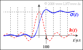
(5) It is obvious that $y_3(t)$ attains its maximum when the ${\rm si}$–function intersects the abscissa for the first time at positive times (see sketch). So, it must hold::
- $$t_{\rm max} = 1/Δf \rm \underline{\: = 100 \: µ s}.$$
- The signal value is obtained according to the table on the information page and is
- $$y_3(t = t_{\rm max}) = 10\hspace{0.1cm}{\rm V} \cdot \big[ {1}/{2} + {1}/{\pi}\cdot {\rm Si} ( \pi )\big]= 10\hspace{0.1cm}{\rm V} \cdot \big[ 0.5 + 0.5895 \big] \hspace{0.15cm}\underline{= 10.895 \hspace{0.1cm}{\rm V}} .$$
- At later times $t$ , $y_3(t)$ slowly adjusts to its final value $10 \ \rm V$.
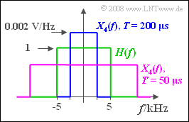
(6) The spectral function $X_4(f)$ is rectangular like $H(f)$ and for $|f| > 2.5 \ \rm kHz$ always zero.
- This means that $Y_4(f ) = X_4(f)$ holds and so does $y_4(t) = x_4(t)$.
- Thus, $y_4(t = 0) \rm \underline{\: = 10 \: \rm V}$.
(7) Due to $T = 50 \ \rm µ s$ , $X_4(f)$ has the width $20 \ \rm kHz$ and the height $0.5 · 10 ^{-3} \ \rm V/Hz$.
- The spectral function $Y_4(f)$ has the same height after being multiplied by $H(f)$ .
- The width $10 \ \rm kHz$ is now determined exclusively by $H(f)$ :
- $$y_4(t) = 0.5 \cdot 10^{-3}\hspace{0.1cm}{ {\rm V} }/{ {\rm Hz} } \cdot 10 \hspace{0.1cm}{\rm kHz} \cdot {\rm si}(\pi \Delta f t ) = 5\hspace{0.1cm}{\rm V} \cdot {\rm si}(\pi \Delta f t )$$
- $$ \Rightarrow \hspace{0.3cm}y_4(t = 0) \hspace{0.15cm}\underline{=5\hspace{0.1cm}{\rm V} }.$$


