Difference between revisions of "Aufgaben:Exercise 2.2: Binary Bipolar Rectangles"
m (Text replacement - "Category:Aufgaben zu Digitalsignalübertragung" to "Category:Digital Signal Transmission: Exercises") |
|||
| (6 intermediate revisions by 2 users not shown) | |||
| Line 1: | Line 1: | ||
| − | {{quiz-Header|Buchseite= | + | {{quiz-Header|Buchseite=Digital_Signal_Transmission/Basics_of_Coded_Transmission |
}} | }} | ||
| − | [[File:P_ID1310__Dig_A_2_2.png|right|frame| | + | [[File:P_ID1310__Dig_A_2_2.png|right|frame|Binary bipolar rectangular signals]] |
| − | + | We assume the following signal: | |
:$$s(t) = \sum_{\nu = -\infty}^{+\infty} a_\nu \cdot g_s ( t - \nu \cdot T) \hspace{0.05cm}.$$ | :$$s(t) = \sum_{\nu = -\infty}^{+\infty} a_\nu \cdot g_s ( t - \nu \cdot T) \hspace{0.05cm}.$$ | ||
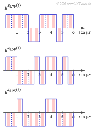
| − | + | The basic transmission pulse $g_{s}(t)$ is always assumed to be rectangular in this exercise, with the NRZ format (blue signal curves in the graph) as well as the RZ format with duty cycle $T_{\rm S}/T = 0.5$ (red signal curves) to be investigated. | |
| − | + | The amplitude coefficients have the following properties: | |
| − | * | + | *They are binary and bipolar: $a_{\nu} \in \{–1, +1\}$. |
| − | * | + | *The symbols within the sequence $\langle a_{\nu }\rangle$ have no statistical ties. |
| − | * | + | *The probabilities for the two possible values $±1$ are with $0 < p < 1$: |
:$${\rm Pr}(a_\nu = +1) \ = \ p,$$ | :$${\rm Pr}(a_\nu = +1) \ = \ p,$$ | ||
:$${\rm Pr}(a_\nu = -1) \ = \ 1 - p \hspace{0.05cm}.$$ | :$${\rm Pr}(a_\nu = -1) \ = \ 1 - p \hspace{0.05cm}.$$ | ||
| − | + | The three signal sections shown in the graph are valid for $p = 0.75$, $p = 0.50$ and $p = 0.25$. | |
| − | + | Throughout this exercise, reference is made to the following descriptive quantities: | |
| − | + | *$m_{a} = \E\big[a_{\nu}\big]$ indicates the linear mean (first order moment) of the amplitude coefficients. | |
| − | *$m_{a} = \E\big[a_{\nu}\big]$ | + | *$m_{2a} = \E\big[a_{\nu}^{2}\big]$ is the power (second order moment). |
| − | *$m_{2a} = \E\big[a_{\nu}^{2}\big]$ | + | *Thus, the variance $\sigma_{a}^{2} = m_{2a} - m_{a}^{2}$ can also be calculated. |
| − | * | + | *The discrete ACF of the amplitude coefficients is $\varphi_{a}(\lambda) = \E\big[a_{\nu} \cdot a_{\nu + \lambda} \big]$. It holds here: |
| − | * | + | :$$\varphi_a(\lambda) = \left\{ \begin{array}{c} m_2 \\ m_1^2 \\ \end{array} \right.\quad \begin{array}{*{1}c} {\rm{for}}\\ {\rm{for}} \\ \end{array} \begin{array}{*{20}c}\lambda = 0, \\ \lambda \ne 0 \hspace{0.05cm}.\\ \end{array}$$ |
| − | :$$\varphi_a(\lambda) = \left\{ \begin{array}{c} m_2 \\ m_1^2 \\ \end{array} \right.\quad \begin{array}{*{1}c} {\rm{ | + | *The energy ACF of the basic transmission pulse is: |
| − | * | + | :$$\varphi^{^{\bullet}}_{g_s}(\tau) = \left\{ \begin{array}{c} s_0^2 \cdot T_{\rm S} \cdot \left( 1 - {|\tau|}/{T_{\rm S}}\right) \\ 0 \\ \end{array} \right.\quad \begin{array}{*{1}c} {\rm{for}}\\ {\rm{for}} \\ \end{array} \begin{array}{*{20}c}|\tau| \le T_{\rm S} \\ |\tau| \ge T_{\rm S} \hspace{0.05cm}.\\ \end{array}$$ |
| − | :$$\varphi^{^{\bullet}}_{g_s}(\tau) = \left\{ \begin{array}{c} s_0^2 \cdot T_{\rm S} \cdot \left( 1 - {|\tau|}/{T_{\rm S}}\right) \\ 0 \\ \end{array} \right.\quad \begin{array}{*{1}c} {\rm{ | + | *Thus, for the total ACF of the transmitted signal, we obtain: |
| − | * | ||
:$$\varphi_s(\tau) = \sum_{\lambda = -\infty}^{+\infty}{1}/{T} \cdot \varphi_a(\lambda)\cdot \varphi^{^{\bullet}}_{g_s}(\tau - \lambda \cdot T)\hspace{0.05cm}.$$ | :$$\varphi_s(\tau) = \sum_{\lambda = -\infty}^{+\infty}{1}/{T} \cdot \varphi_a(\lambda)\cdot \varphi^{^{\bullet}}_{g_s}(\tau - \lambda \cdot T)\hspace{0.05cm}.$$ | ||
| − | * | + | *The power-spectral density ${\it \Phi}_{s}(f)$ is the Fourier transform of the ACF $\varphi_{s}(\tau)$. |
| − | |||
| − | |||
| − | |||
| − | + | Note: The exercise belongs to the chapter [[Digital_Signal_Transmission/Basics_of_Coded_Transmission|"Basics of Coded Transmission"]]. | |
| − | |||
| − | === | + | ===Questions=== |
<quiz display=simple> | <quiz display=simple> | ||
| − | { | + | {Which of the three signals shown are redundancy-free? |
|type="[]"} | |type="[]"} | ||
- $s_{0.75}(t)$, | - $s_{0.75}(t)$, | ||
| Line 50: | Line 45: | ||
| − | { | + | {What is the second order moment ("power") $m_{2a}= \E\big[a_{\nu}^{2}\big]$ of the amplitude coefficients as a function of $p$? |
|type="{}"} | |type="{}"} | ||
$p = 0.75\text{:} \hspace{0.4cm} m_{2a} \ = \ $ { 1 3% } | $p = 0.75\text{:} \hspace{0.4cm} m_{2a} \ = \ $ { 1 3% } | ||
| Line 56: | Line 51: | ||
$p = 0.25\text{:} \hspace{0.4cm} m_{2a} \ = \ $ { 1 3% } | $p = 0.25\text{:} \hspace{0.4cm} m_{2a} \ = \ $ { 1 3% } | ||
| − | { | + | {Calculate the first order moment ("linear mean") $m_{a}= \E\big[a_{\nu}\big]$ in relation to $p$. |
|type="{}"} | |type="{}"} | ||
$p = 0.75\text{:} \hspace{0.4cm} m_{a} \ = \ $ { 0.5 3% } | $p = 0.75\text{:} \hspace{0.4cm} m_{a} \ = \ $ { 0.5 3% } | ||
| Line 62: | Line 57: | ||
$p = 0.25\text{:} \hspace{0.4cm} m_{a} \ = \ $ { -0.515--0.485 } | $p = 0.25\text{:} \hspace{0.4cm} m_{a} \ = \ $ { -0.515--0.485 } | ||
| − | { | + | {What is the variance $\sigma_{a}^{2}$ of the amplitude coefficients? |
|type="{}"} | |type="{}"} | ||
$p = 0.75\text{:} \hspace{0.4cm} \sigma_{a}^{2} \ = \ $ { 0.75 3% } | $p = 0.75\text{:} \hspace{0.4cm} \sigma_{a}^{2} \ = \ $ { 0.75 3% } | ||
| Line 68: | Line 63: | ||
$p = 0.25\text{:} \hspace{0.4cm} \sigma_{a}^{2} \ = \ $ { 0.75 3% } | $p = 0.25\text{:} \hspace{0.4cm} \sigma_{a}^{2} \ = \ $ { 0.75 3% } | ||
| − | { | + | {Let $p = 0.5$ hold initially. Sketch the ACF $\varphi_{s}(\tau)$ for the NRZ and RZ basic transmission pulses and evaluate the following statements: |
|type="[]"} | |type="[]"} | ||
| − | + | + | + The ACF is triangular in both cases. |
| − | + | + | + The PSD is ${\rm sinc}^{2}$–shaped in both cases. |
| − | - | + | -The PSD area is the same in both cases. |
| − | - | + | -In the case of RZ pulses, ${\it \Phi}_{s}(f)$ involves additional Dirac delta functions. |
| − | { | + | {Let be $p = 0.75$. Sketch the ACF for the NRZ basic pulse and evaluate the following statements: |
|type="[]"} | |type="[]"} | ||
| − | + | + | + The ACF consists of a triangle and a DC component. |
| − | + | + | + The PSD consists of a ${\rm sinc}^{2}$ component and a Dirac delta function. |
| − | - | + | -The Dirac delta function has the weight $s_{0}^{2}$. |
| − | + | + | +With $p = 0.25$, the same power-spectral density is obtained. |
| − | { | + | {Let be $p = 0.75$. Sketch the ACF for the RZ basic pulse and evaluate the following statements: |
|type="[]"} | |type="[]"} | ||
| − | + | + | + Again, the PSD contains a ${\rm sinc}^{2}$–shaped component. |
| − | + | + | + At the same time, there are still infinitely many Dirac delta lines in the PSD. |
</quiz> | </quiz> | ||
| − | === | + | ===Solution=== |
{{ML-Kopf}} | {{ML-Kopf}} | ||
| − | '''(1)''' | + | '''(1)''' A digital signal is said to be redundancy-free if |
| − | * | + | *the amplitude coefficients do not depend on each other (this was assumed here), |
| − | * | + | *all possible amplitude coefficients are equally probable. |
| − | In | + | In this sense, $s_{0.5}(t)$ is a redundancy-free signal ⇒ <u>solution 2</u>. |
| − | * | + | *Thus, here the entropy (the average information content per transmitted binary symbol) is at most equal to the decision content: |
| − | :$$H_{\rm max} = {1}/{2}\cdot {\rm log}_2 (2)+{1}/{2}\cdot {\rm log}_2 (2) = 1 \,\,{\rm bit/ | + | :$$H_{\rm max} = {1}/{2}\cdot {\rm log}_2 (2)+{1}/{2}\cdot {\rm log}_2 (2) = 1 \,\,{\rm bit/binary\ symbol} \hspace{0.05cm}.$$ |
| − | * | + | *In contrast, the entropies of the other two binary signals are: |
:$$H = \ \frac{3}{4}\cdot {\rm log}_2 (\frac{4}{3})+ \frac{1}{4}\cdot {\rm log}_2 (4) | :$$H = \ \frac{3}{4}\cdot {\rm log}_2 (\frac{4}{3})+ \frac{1}{4}\cdot {\rm log}_2 (4) | ||
= \left( \frac{3}{4} + \frac{1}{4}\right)\cdot {\rm log}_2 (4) - | = \left( \frac{3}{4} + \frac{1}{4}\right)\cdot {\rm log}_2 (4) - | ||
\frac{3}{4}\cdot{\rm log}_2 (3) =$$ | \frac{3}{4}\cdot{\rm log}_2 (3) =$$ | ||
:$$ \hspace{0.5cm} = \ 2 - \frac{3}{4}\cdot{\rm log}_2 (3) = | :$$ \hspace{0.5cm} = \ 2 - \frac{3}{4}\cdot{\rm log}_2 (3) = | ||
| − | 0.811 \,\,{\rm bit/ | + | 0.811 \,\,{\rm bit/binary\ symbol} \hspace{0.05cm}.$$ |
| − | * | + | *From this, the relative redundancy of these signals is: |
:$$r = \frac{H_{\rm max} - H}{H_{\rm max}}\hspace{0.15cm} \approx 18.9\%\hspace{0.05cm}.$$ | :$$r = \frac{H_{\rm max} - H}{H_{\rm max}}\hspace{0.15cm} \approx 18.9\%\hspace{0.05cm}.$$ | ||
| − | '''(2)''' | + | '''(2)''' The second order moment ("power") is equal to $m_{2a} = 1$ independent of $p$: |
:$$m_{2a}={\rm E}[a_\nu^2] = p \cdot (+1)^2 + (1-p)\cdot (-1)^2 \hspace{0.15cm}\underline { = 1 \hspace{0.05cm}}.$$ | :$$m_{2a}={\rm E}[a_\nu^2] = p \cdot (+1)^2 + (1-p)\cdot (-1)^2 \hspace{0.15cm}\underline { = 1 \hspace{0.05cm}}.$$ | ||
| − | '''(3)''' | + | '''(3)''' For the first order moment ("linear mean") we get: |
:$$m_{a}={\rm E}[a_\nu] = p \cdot (+1) + (1-p)\cdot (-1) = 2 p -1 \hspace{0.05cm}.$$ | :$$m_{a}={\rm E}[a_\nu] = p \cdot (+1) + (1-p)\cdot (-1) = 2 p -1 \hspace{0.05cm}.$$ | ||
:$$\Rightarrow \hspace{0.3cm} p = 0.75\text{:} \hspace{0.4cm} m_{a}\hspace{0.15cm}\underline {=0.50},\hspace{0.2cm} p = 0.50\text{:} \hspace{0.4cm} m_{a}\hspace{0.15cm}\underline {=0},\hspace{0.2cm} p = 0.25\text{:} \hspace{0.4cm} m_{a}\hspace{0.15cm}\underline { =-0.50 \hspace{0.05cm}}.$$ | :$$\Rightarrow \hspace{0.3cm} p = 0.75\text{:} \hspace{0.4cm} m_{a}\hspace{0.15cm}\underline {=0.50},\hspace{0.2cm} p = 0.50\text{:} \hspace{0.4cm} m_{a}\hspace{0.15cm}\underline {=0},\hspace{0.2cm} p = 0.25\text{:} \hspace{0.4cm} m_{a}\hspace{0.15cm}\underline { =-0.50 \hspace{0.05cm}}.$$ | ||
| − | '''(4)''' | + | '''(4)''' Using the results from ( '''(2)''' and '''(4)''', we obtain: |
:$$p = 0.75\text{:} \hspace{0.4cm} \sigma_{a}^2 \hspace{0.15cm}\underline {=0.75},$$ | :$$p = 0.75\text{:} \hspace{0.4cm} \sigma_{a}^2 \hspace{0.15cm}\underline {=0.75},$$ | ||
:$$ p = 0.50\text{:} \hspace{0.4cm} \sigma_{a}^2\hspace{0.15cm} \underline { =1.00 \hspace{0.05cm}},$$ | :$$ p = 0.50\text{:} \hspace{0.4cm} \sigma_{a}^2\hspace{0.15cm} \underline { =1.00 \hspace{0.05cm}},$$ | ||
| Line 124: | Line 119: | ||
| − | [[File:P_ID1311__Dig_A_2_2e.png|right|frame| | + | [[File:P_ID1311__Dig_A_2_2e.png|right|frame|ACF with equal symbol probabilities]] |
| − | '''(5)''' | + | '''(5)''' Only the <u>first two statements</u> are correct: |
| − | * | + | *For $p = 0.5$, $\varphi_{a}(\lambda = 0) = 1$ and $\varphi_{a}(\lambda \neq 0) = 0$. It follows that: |
:$$\varphi_s(\tau) = \frac{1}{T} \cdot \varphi^{^{\bullet}}_{gs}(\tau )\hspace{0.05cm}.$$ | :$$\varphi_s(\tau) = \frac{1}{T} \cdot \varphi^{^{\bullet}}_{gs}(\tau )\hspace{0.05cm}.$$ | ||
| − | * | + | *This results in a triangular ACF and a ${\rm sinc}^{2}$–shaped PSD for both the NRZ and RZ basic pulses. |
| − | * | + | *The area under the PSD is smaller by a factor of $T_{\rm S}/T$ for the RZ pulse than for the NRZ pulse, <br>since the ACF values also differ by this factor at $\tau = 0$. |
| − | * | + | *The PSD is continuous in both cases because the ACF does not contain a DC component or periodic components. |
| − | [[File:P_ID1330__Dig_A_2_2f.png|right|frame| | + | [[File:P_ID1330__Dig_A_2_2f.png|right|frame|ACF with unequal symbol probabilities]] |
| − | '''(6)''' | + | '''(6)''' <u>All statements except the third</u> are correct: |
| − | * | + | *For $p = 0.75$, the ACF $\varphi_{s}(\tau)$ is composed of infinitely many triangular functions, all of which have the same height $s_{0}^{2}/4$ except for the middle triangle around $\tau = 0$. |
| − | * | + | *According to the sketch, one can combine all these triangle functions into a DC component of height $m_{a}^{2} \cdot s_{0}^{2} = s_{0}^{2}/4$ and a single triangle around $\tau = 0$ with height $\sigma_{a}^{2} \cdot s_{0}^{2} = 3/4 · s_{0}^{2}$. |
| − | * | + | *In the PSD, this leads to a continuous ${\rm sinc}^{2}$–shaped component and a Dirac delta function at $f = 0$. The weight of this Dirac is $s_{0}^{2}/4$. |
| − | * | + | *For $p = 0.25$ we get the same ACF as with $p = 0.75$, since both the second order moment $m_{2a} = 1$ and $m_{a}^{2} = 0.25$ coincide. Thus, of course, the power-spectral densities also match. |
| − | [[File:P_ID1331__Dig_A_2_2g.png|right|frame| | + | [[File:P_ID1331__Dig_A_2_2g.png|right|frame|ACF for RZ rectangular pulses]] |
| − | '''(7)''' <u> | + | '''(7)''' <u>Both proposed solutions are correct:</u>: |
| − | * | + | *With the RZ duty cycle $T_{\rm S}/T = 0.5$ the sketched ACF is obtained, which can also be represented by a periodic triangular function of height $s_{0}^{2}/8$ (red filling) and a single triangular pulse of height $3/8 \cdot s_{0}^{2}$ (green filling). |
| − | * | + | *This non-periodic component leads to a continuous-valued, ${\rm sinc}^{2}$–shaped PSD with zeros at multiples of $2/T$. |
| − | * | + | *The periodic triangular ACF causes Dirac delta functions in the PSD at multiples of $1/T$. |
| − | * | + | *However, due to the antimetry of the periodic component, the Dirac delta functions at multiples of $2/T$ each have weight $0$. |
| − | * | + | *The weights of the Dirac delta functions at distance $1/T$ are proportional to the continuous PSD component. |
| Line 155: | Line 150: | ||
| − | [[Category:Digital Signal Transmission: Exercises|^2.1 | + | [[Category:Digital Signal Transmission: Exercises|^2.1 Basics of Coded Transmission^]] |
Latest revision as of 19:02, 13 May 2022
We assume the following signal:
- $$s(t) = \sum_{\nu = -\infty}^{+\infty} a_\nu \cdot g_s ( t - \nu \cdot T) \hspace{0.05cm}.$$
The basic transmission pulse $g_{s}(t)$ is always assumed to be rectangular in this exercise, with the NRZ format (blue signal curves in the graph) as well as the RZ format with duty cycle $T_{\rm S}/T = 0.5$ (red signal curves) to be investigated.
The amplitude coefficients have the following properties:
- They are binary and bipolar: $a_{\nu} \in \{–1, +1\}$.
- The symbols within the sequence $\langle a_{\nu }\rangle$ have no statistical ties.
- The probabilities for the two possible values $±1$ are with $0 < p < 1$:
- $${\rm Pr}(a_\nu = +1) \ = \ p,$$
- $${\rm Pr}(a_\nu = -1) \ = \ 1 - p \hspace{0.05cm}.$$
The three signal sections shown in the graph are valid for $p = 0.75$, $p = 0.50$ and $p = 0.25$.
Throughout this exercise, reference is made to the following descriptive quantities:
- $m_{a} = \E\big[a_{\nu}\big]$ indicates the linear mean (first order moment) of the amplitude coefficients.
- $m_{2a} = \E\big[a_{\nu}^{2}\big]$ is the power (second order moment).
- Thus, the variance $\sigma_{a}^{2} = m_{2a} - m_{a}^{2}$ can also be calculated.
- The discrete ACF of the amplitude coefficients is $\varphi_{a}(\lambda) = \E\big[a_{\nu} \cdot a_{\nu + \lambda} \big]$. It holds here:
- $$\varphi_a(\lambda) = \left\{ \begin{array}{c} m_2 \\ m_1^2 \\ \end{array} \right.\quad \begin{array}{*{1}c} {\rm{for}}\\ {\rm{for}} \\ \end{array} \begin{array}{*{20}c}\lambda = 0, \\ \lambda \ne 0 \hspace{0.05cm}.\\ \end{array}$$
- The energy ACF of the basic transmission pulse is:
- $$\varphi^{^{\bullet}}_{g_s}(\tau) = \left\{ \begin{array}{c} s_0^2 \cdot T_{\rm S} \cdot \left( 1 - {|\tau|}/{T_{\rm S}}\right) \\ 0 \\ \end{array} \right.\quad \begin{array}{*{1}c} {\rm{for}}\\ {\rm{for}} \\ \end{array} \begin{array}{*{20}c}|\tau| \le T_{\rm S} \\ |\tau| \ge T_{\rm S} \hspace{0.05cm}.\\ \end{array}$$
- Thus, for the total ACF of the transmitted signal, we obtain:
- $$\varphi_s(\tau) = \sum_{\lambda = -\infty}^{+\infty}{1}/{T} \cdot \varphi_a(\lambda)\cdot \varphi^{^{\bullet}}_{g_s}(\tau - \lambda \cdot T)\hspace{0.05cm}.$$
- The power-spectral density ${\it \Phi}_{s}(f)$ is the Fourier transform of the ACF $\varphi_{s}(\tau)$.
Note: The exercise belongs to the chapter "Basics of Coded Transmission".
Questions
Solution
- the amplitude coefficients do not depend on each other (this was assumed here),
- all possible amplitude coefficients are equally probable.
In this sense, $s_{0.5}(t)$ is a redundancy-free signal ⇒ solution 2.
- Thus, here the entropy (the average information content per transmitted binary symbol) is at most equal to the decision content:
- $$H_{\rm max} = {1}/{2}\cdot {\rm log}_2 (2)+{1}/{2}\cdot {\rm log}_2 (2) = 1 \,\,{\rm bit/binary\ symbol} \hspace{0.05cm}.$$
- In contrast, the entropies of the other two binary signals are:
- $$H = \ \frac{3}{4}\cdot {\rm log}_2 (\frac{4}{3})+ \frac{1}{4}\cdot {\rm log}_2 (4) = \left( \frac{3}{4} + \frac{1}{4}\right)\cdot {\rm log}_2 (4) - \frac{3}{4}\cdot{\rm log}_2 (3) =$$
- $$ \hspace{0.5cm} = \ 2 - \frac{3}{4}\cdot{\rm log}_2 (3) = 0.811 \,\,{\rm bit/binary\ symbol} \hspace{0.05cm}.$$
- From this, the relative redundancy of these signals is:
- $$r = \frac{H_{\rm max} - H}{H_{\rm max}}\hspace{0.15cm} \approx 18.9\%\hspace{0.05cm}.$$
(2) The second order moment ("power") is equal to $m_{2a} = 1$ independent of $p$:
- $$m_{2a}={\rm E}[a_\nu^2] = p \cdot (+1)^2 + (1-p)\cdot (-1)^2 \hspace{0.15cm}\underline { = 1 \hspace{0.05cm}}.$$
(3) For the first order moment ("linear mean") we get:
- $$m_{a}={\rm E}[a_\nu] = p \cdot (+1) + (1-p)\cdot (-1) = 2 p -1 \hspace{0.05cm}.$$
- $$\Rightarrow \hspace{0.3cm} p = 0.75\text{:} \hspace{0.4cm} m_{a}\hspace{0.15cm}\underline {=0.50},\hspace{0.2cm} p = 0.50\text{:} \hspace{0.4cm} m_{a}\hspace{0.15cm}\underline {=0},\hspace{0.2cm} p = 0.25\text{:} \hspace{0.4cm} m_{a}\hspace{0.15cm}\underline { =-0.50 \hspace{0.05cm}}.$$
(4) Using the results from ( (2) and (4), we obtain:
- $$p = 0.75\text{:} \hspace{0.4cm} \sigma_{a}^2 \hspace{0.15cm}\underline {=0.75},$$
- $$ p = 0.50\text{:} \hspace{0.4cm} \sigma_{a}^2\hspace{0.15cm} \underline { =1.00 \hspace{0.05cm}},$$
- $$ p = 0.25\text{:} \hspace{0.4cm} \sigma_{a}^2 \hspace{0.15cm}\underline {=0.75}.$$
(5) Only the first two statements are correct:
- For $p = 0.5$, $\varphi_{a}(\lambda = 0) = 1$ and $\varphi_{a}(\lambda \neq 0) = 0$. It follows that:
- $$\varphi_s(\tau) = \frac{1}{T} \cdot \varphi^{^{\bullet}}_{gs}(\tau )\hspace{0.05cm}.$$
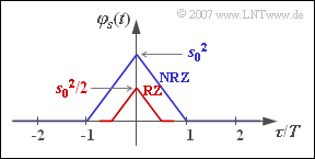
- This results in a triangular ACF and a ${\rm sinc}^{2}$–shaped PSD for both the NRZ and RZ basic pulses.
- The area under the PSD is smaller by a factor of $T_{\rm S}/T$ for the RZ pulse than for the NRZ pulse,
since the ACF values also differ by this factor at $\tau = 0$. - The PSD is continuous in both cases because the ACF does not contain a DC component or periodic components.
(6) All statements except the third are correct:
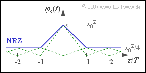
- For $p = 0.75$, the ACF $\varphi_{s}(\tau)$ is composed of infinitely many triangular functions, all of which have the same height $s_{0}^{2}/4$ except for the middle triangle around $\tau = 0$.
- According to the sketch, one can combine all these triangle functions into a DC component of height $m_{a}^{2} \cdot s_{0}^{2} = s_{0}^{2}/4$ and a single triangle around $\tau = 0$ with height $\sigma_{a}^{2} \cdot s_{0}^{2} = 3/4 · s_{0}^{2}$.
- In the PSD, this leads to a continuous ${\rm sinc}^{2}$–shaped component and a Dirac delta function at $f = 0$. The weight of this Dirac is $s_{0}^{2}/4$.
- For $p = 0.25$ we get the same ACF as with $p = 0.75$, since both the second order moment $m_{2a} = 1$ and $m_{a}^{2} = 0.25$ coincide. Thus, of course, the power-spectral densities also match.
(7) Both proposed solutions are correct::
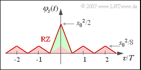
- With the RZ duty cycle $T_{\rm S}/T = 0.5$ the sketched ACF is obtained, which can also be represented by a periodic triangular function of height $s_{0}^{2}/8$ (red filling) and a single triangular pulse of height $3/8 \cdot s_{0}^{2}$ (green filling).
- This non-periodic component leads to a continuous-valued, ${\rm sinc}^{2}$–shaped PSD with zeros at multiples of $2/T$.
- The periodic triangular ACF causes Dirac delta functions in the PSD at multiples of $1/T$.
- However, due to the antimetry of the periodic component, the Dirac delta functions at multiples of $2/T$ each have weight $0$.
- The weights of the Dirac delta functions at distance $1/T$ are proportional to the continuous PSD component.


