Basics of Coded Transmission

1 # OVERVIEW OF THE SECOND MAIN CHAPTER #
2 Information content – Entropy – Redundancy
3 Source coding – Channel coding – Line coding
4 System model and description variables
5 ACF calculation of a digital signal
6 PSD calculation of a digital signal
7 ACF and PSD for bipolar binary signals
8 ACF and PSD for unipolar binary signals
9 Exercises for the chapter

# OVERVIEW OF THE SECOND MAIN CHAPTER #

The second main chapter deals with so-called transmission coding, which is sometimes also referred to as "line coding" in literature. In this process, an adaptation of the digital transmitted signal to the characteristics of the transmission channel is achieved through the targeted addition of redundancy. In detail, the following are dealt with:

Some basic concepts of information theory such as »information content« and »entropy«,
the »auto-correlation function« and the »power-spectral densities« of digital signals,
the »redundancy-free coding« which leads to a non-binary transmitted signal,
the calculation of »symbol and bit error probability« for »multilevel systems« ,
the so-called »4B3T codes« as an important example of »block-wise coding«, and
the »pseudo-ternary codes«, each of which realizes symbol-wise coding.

The description is in baseband throughout and some simplifying assumptions (among others: no intersymbol interfering) are still made.

Information content – Entropy – Redundancy

We assume an $M$–level digital source that outputs the following source signal:

$$q(t) = \sum_{(\nu)} a_\nu \cdot {\rm \delta} ( t - \nu \cdot T)\hspace{0.3cm}{\rm with}\hspace{0.3cm}a_\nu \in \{ a_1, \text{...} \ , a_\mu , \text{...} \ , a_{ M}\}.$$

The source symbol sequence $\langle q_\nu \rangle$ is thus mapped to the sequence $\langle a_\nu \rangle$ of the dimensionless amplitude coefficients.

Simplifying, first for the time indexing variable $\nu = 1$, ... , $N$ is set, while the ensemble indexing variable $\mu$ can assume values between $1$ and level number $M$.

If the $\nu$–th sequence element is equal to $a_\mu$, its information content can be calculated with probability $p_{\nu\mu} = {\rm Pr}(a_\nu = a_\mu)$ as follows:

$$I_\nu = \log_2 \ (1/p_{\nu \mu})= {\rm ld} \ (1/p_{\nu \mu}) \hspace{1cm}\text{(unit: bit)}\hspace{0.05cm}.$$

The logarithm to the base 2 ⇒ $\log_2(x)$ is often also called ${\rm ld}(x)$ ⇒ "logarithm dualis". With the numerical evaluation the reference unit "bit" (from: "binary digit" ) is added. With the tens logarithm $\lg(x)$ and the natural logarithm $\ln(x)$ applies:

$${\rm log_2}(x) = \frac{{\rm lg}(x)}{{\rm lg}(2)}= \frac{{\rm ln}(x)}{{\rm ln}(2)}\hspace{0.05cm}.$$

According to this definition, which goes back to "Claude E. Shannon", the smaller the probability of occurrence of a symbol, the greater its information content.

$\text{Definition:}$ Entropy is the "average information content" of a sequence element ("symbol").

This important information-theoretical quantity can be determined as a time average as follows:

$$H = \lim_{N \to \infty} \frac{1}{N} \cdot \sum_{\nu = 1}^N I_\nu = \lim_{N \to \infty} \frac{1}{N} \cdot \sum_{\nu = 1}^N \hspace{0.1cm}{\rm log_2}\hspace{0.05cm} \ (1/p_{\nu \mu}) \hspace{1cm}\text{(unit: bit)}\hspace{0.05cm}.$$

Of course, the entropy can also be calculated by ensemble averaging (over the symbol set).

Note:

If the sequence elements $a_\nu$ are statistically independent of each other, the probabilities $p_{\nu\mu} = p_{\mu}$ are independent of $\nu$ and we obtain in this special case:

$$H = \sum_{\mu = 1}^M p_{ \mu} \cdot {\rm log_2}\hspace{0.1cm} \ (1/p_{\mu})\hspace{0.05cm}.$$

If, on the other hand, there are statistical bindings between neighboring amplitude coefficients $a_\nu$, the more complicated equation according to the above definition must be used for entropy calculation.

$\text{Definitions:}$

The maximum value of entropy ⇒ decision content is obtained whenever the $M$ occurrence probabilities (of the statistically independent symbols) are all equal $(p_{\mu} = 1/M)$:

$$H_{\rm max} = \sum_{\mu = 1}^M \hspace{0.1cm}\frac{1}{M} \cdot {\rm log_2} (M) = {\rm log_2} (M) \cdot \sum_{\mu = 1}^M \hspace{0.1cm} \frac{1}{M} = {\rm log_2} (M) \hspace{1cm}\text{(unit: bit)}\hspace{0.05cm}.$$

The relative redundancy is then the following quotient:

$$r = \frac{H_{\rm max}-H}{H_{\rm max} }.$$

Since $0 \le H \le H_{\rm max}$ always holds, the relative redundancy can take values between $0$ and $1$ (including these limits).

From the derivation of these descriptive quantities, it is obvious that a redundancy-free $(r=0)$ digital signal must satisfy the following properties:

The amplitude coefficients $a_\nu$ are statistically independent ⇒ $p_{\nu\mu} = {\rm Pr}(a_\nu = a_\mu)$ is identical for all $\nu$.
The $M$ possible coefficients $a_\mu$ occur with equal probability $p_\mu = 1/M$.

$\text{Example 1:}$ If one analyzes a German text on the basis of $M = 32$ characters:

$$\text{a, ... , z, ä, ö, ü, ß, spaces, punctuation, no distinction between upper and lower case},$$

the result is the decision content $H_{\rm max} = 5 \ \rm bit/symbol$. Due to

the different frequencies $($for example, "e" occurs significantly more often than "u"$)$, and
statistical ties $($for example "q" is followed by the letter "u" much more often than "e"$)$,

according to "Karl Küpfmüller", the entropy of the German language is only $H = 1.3 \ \rm bit/character$. This results in a relative redundancy of $r \approx (5 - 1.3)/5 = 74\%$.

For English texts, "Claude Shannon" has given the entropy as $H = 1 \ \rm bit/character$ and the relative redundancy as $r \approx 80\%$.

Source coding – Channel coding – Line coding

"Coding" is the conversion of the source symbol sequence $\langle q_\nu \rangle$ with symbol set size $M_q$ into an encoder symbol sequence $\langle c_\nu \rangle$ with symbol set size $M_c$. Usually, coding manipulates the redundancy contained in a digital signal. Often – but not always – $M_q$ and $M_c$ are different.

A distinction is made between different types of coding depending on the target direction:

The task of source coding is redundancy reduction for data compression, as applied for example in image coding. By exploiting statistical ties between the individual points of an image or between the brightness values of a point at different times (in the case of moving image sequences), methods can be developed that lead to a noticeable reduction in the amount of data (measured in "bit" or "byte"), while maintaining virtually the same (subjective) image quality. A simple example of this is "differential pulse code modulation" $\rm (DPCM)$.

On the other hand, with channel coding a noticeable improvement in the transmission behavior is achieved by using a redundancy specifically added at the transmitter to detect and correct transmission errors at the receiver end. Such codes, the most important of which are block codes, convolutional codes and turbo codes, are particularly important in the case of heavily disturbed channels. The greater the relative redundancy of the encoded signal, the better the correction properties of the code, albeit at a reduced user data rate.

Line coding is used to adapt the transmitted signal to the spectral characteristics of the transmission channel and the receiving equipment by recoding the source symbols. For example, in the case of a channel with the frequency response characteristic $H_{\rm K}(f=0) = 0$, over which consequently no DC signal can be transmitted, transmission coding must ensure that the encoder symbol sequence contains neither a long $\rm L$ sequence nor a long $\rm H$ sequence.

In the current book "Digital Signal Transmission" we deal exclusively with this last, transmission-technical aspect.

"Channel Coding" has its own book dedicated to it in our learning tutorial.
Source coding is covered in detail in the book "Information Theory" (main chapter 2).
"Speech coding" – described in the book "Examples of Communication Systems" – is a special form of source coding.

System model and description variables

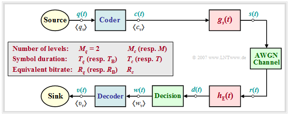
In the following we always assume the block diagram sketched on the right and the following agreements:

Block diagram for the description of multilevel and coded transmission systems

Let the digital source signal $q(t)$ be binary $(M_q = 2)$ and redundancy-free $(H_q = 1 \ \rm bit/symbol)$.

With the symbol duration $T_q$ results for the symbol rate of the source:

$$R_q = {H_{q}}/{T_q}= {1}/{T_q}\hspace{0.05cm}.$$

Because of $M_q = 2$, in the following we also refer to $T_q$ as the "bit duration" and $R_q$ as the "bit rate".

For the comparison of transmission systems with different coding, $T_q$ and $R_q$ are always assumed to be constant. Note: In later chapters we use $T_{\rm B}=T_q$ and $R_{\rm B}=R_q$ for this purpose.

The encoded signal $c(t)$ and also the transmitted signal $s(t)$ after pulse shaping with $g_s(t)$ have the level number $M_c$, the symbol duration $T_c$ and the symbol rate $1/T_c$. The equivalent bit rate is

$$R_c = {{\rm log_2} (M_c)}/{T_c} \ge R_q \hspace{0.05cm}.$$

The equal sign is only valid for the "redundancy-free codes" $(r_c = 0)$.
Otherwise, we obtain for the relative code redundancy:

$$r_c =({R_c - R_q})/{R_c} = 1 - R_q/{R_c} \hspace{0.05cm}.$$

Notes on nomenclature:

In the context of transmission codes, $R_c$ always indicates in our tutorial the equivalent bit rate of the encoded signal with unit "bit/s".
In the literature on channel coding, $R_c$ is often used to denote the dimensionless code rate $1 - r_c$ .
$R_c = 1 $ then indicates a redundancy-free code, while $R_c = 1/3 $ indicates a code with the relative redundancy $r_c = 2/3 $.

$\text{Example 2:}$ In the so-called "4B3T codes",

four binary symbols $(m_q = 4, \ M_q= 2)$ are each represented by
three ternary symbols $(m_c = 3, \ M_c= 3)$.

Because of $4 \cdot T_q = 3 \cdot T_c$ holds:

$$R_q = {1}/{T_q}, \hspace{0.1cm} R_c = { {\rm log_2} (3)} \hspace{-0.05cm} /{T_c} = {3/4 \cdot {\rm log_2} (3)} \hspace{-0.05cm}/{T_q}$$

$$\Rightarrow \hspace{0.3cm}r_c =3/4\cdot {\rm log_2} (3) \hspace{-0.05cm}- \hspace{-0.05cm}1 \approx 15.9\, \% \hspace{0.05cm}.$$

Detailed information about the 4B3T codes can be found in the "chapter of the same name".

ACF calculation of a digital signal

To simplify the notation, $M_c = M$ and $T_c = T$ is set in the following. Thus, for the transmitted signal $s(t)$ in the case of an unlimited-time sybol sequence with $a_\nu \in \{ a_1,$ ... , $a_M\}$ can be written:

Two different binary bipolar transmitted signals

$$s(t) = \sum_{\nu = -\infty}^{+\infty} a_\nu \cdot g_s ( t - \nu \cdot T) \hspace{0.05cm}.$$

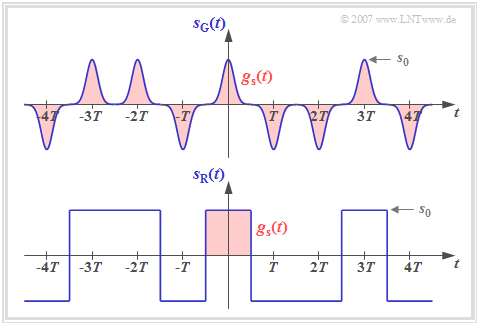
This signal representation includes both the source statistics $($amplitude coefficients $a_\nu$) and the transmission pulse shape $g_s(t)$. The diagram shows two binary bipolar transmitted signals $s_{\rm G}(t)$ and $s_{\rm R}(t)$ with the same amplitude coefficients $a_\nu$, which thus differ only by the basic transmission pulse $g_s(t)$.

It can be seen from this figure that a digital signal is generally non-stationary:

For the transmitted signal $s_{\rm G}(t)$ with narrow Gaussian pulses, the "non-stationarity" is obvious, since, for example, at multiples of $T$ the variance is $\sigma_s^2 = s_0^2$, while exactly in between $\sigma_s^2 \approx 0$ holds.

Also the signal $s_{\rm R}(t)$ with NRZ rectangular pulses is non–stationary in a strict sense, because here the moments at the bit boundaries differ with respect to all other instants. For example, $s_{\rm R}(t = \pm T/2)=0$.

$\text{Definition:}$

A random process whose moments $m_k(t) = m_k(t+ \nu \cdot T)$ repeat periodically with $T$ is called cyclostationary.
In this implicit definition, $k$ and $\nu$ have integer values .

Many of the rules valid for "ergodic processes" can also be applied to "cycloergodic" (and hence to "cyclostationary") processes with only minor restrictions.

In particular, for the "auto-correlation function" $\rm (ACF)$ of such random processes with sample signal $s(t)$ holds:

$$\varphi_s(\tau) = {\rm E}\big [s(t) \cdot s(t + \tau)\big ] \hspace{0.05cm}.$$

With the above equation of the transmitted signal, the ACF as a time average can also be written as follows:

$$\varphi_s(\tau) = \sum_{\lambda = -\infty}^{+\infty}\frac{1}{T} \cdot \lim_{N \to \infty} \frac{1}{2N +1} \cdot \sum_{\nu = -N}^{+N} a_\nu \cdot a_{\nu + \lambda} \cdot \int_{-\infty}^{+\infty} g_s ( t ) \cdot g_s ( t + \tau - \lambda \cdot T)\,{\rm d} t \hspace{0.05cm}.$$

Since the limit, integral and sum may be interchanged, with the substitutions

$$N = T_{\rm M}/(2T), \hspace{0.5cm}\lambda = \kappa- \nu,\hspace{0.5cm}t - \nu \cdot T \to T$$

for this can also be written:

$$\varphi_s(\tau) = \lim_{T_{\rm M} \to \infty}\frac{1}{T_{\rm M}} \cdot \int_{-T_{\rm M}/2}^{+T_{\rm M}/2} \sum_{\nu = -\infty}^{+\infty} \sum_{\kappa = -\infty}^{+\infty} a_\nu \cdot g_s ( t - \nu \cdot T ) \cdot a_\kappa \cdot g_s ( t + \tau - \kappa \cdot T ) \,{\rm d} t \hspace{0.05cm}.$$

Now the following quantities are introduced for abbreviation:

$\text{Definitions:}$

The discrete ACF of the amplitude coefficients provides statements about the linear statistical bonds of the amplitude coefficients $a_{\nu}$ and $a_{\nu + \lambda}$ and has no unit:

$$\varphi_a(\lambda) = \lim_{N \to \infty} \frac{1}{2N +1} \cdot \sum_{\nu = -\infty}^{+\infty} a_\nu \cdot a_{\nu + \lambda} \hspace{0.05cm}.$$

The energy ACF of the basic transmission pulse is defined similarly to the general (power) auto-correlation function. It is marked with a dot:

$$\varphi^{^{\bullet} }_{gs}(\tau) = \int_{-\infty}^{+\infty} g_s ( t ) \cdot g_s ( t + \tau)\,{\rm d} t \hspace{0.05cm}.$$

⇒ Since $g_s(t)$ is "energy-limited", the division by $T_{\rm M}$ and the boundary transition can be omitted.

For the auto-correlation function of a digital signal $s(t)$ holds in general:

$$\varphi_s(\tau) = \sum_{\lambda = -\infty}^{+\infty}{1}/{T} \cdot \varphi_a(\lambda)\cdot\varphi^{^{\bullet} }_{gs}(\tau - \lambda \cdot T)\hspace{0.05cm}.$$

⇒ $s(t)$ can be binary or multilevel, unipolar or bipolar, redundancy-free or redundant (line-coded). The pulse shape is taken into account by the energy ACF.

Note:

If the digital signal $s(t)$ describes a voltage waveform,

the energy ACF of the basic transmission pulse $g_s(t)$ has the unit $\rm V^2s$,
the auto-correlation function $\varphi_s(\tau)$ of the digital signal $s(t)$ has the unit $\rm V^2$ $($each related to the resistor $1 \ \rm \Omega)$.

In the strict sense of system theory, one would have to define the ACF of the amplitude coefficients as follows:

$$\varphi_{a , \hspace{0.08cm}\delta}(\tau) = \sum_{\lambda = -\infty}^{+\infty} \varphi_a(\lambda)\cdot \delta(\tau - \lambda \cdot T)\hspace{0.05cm}.$$

⇒ Thus, the above equation would be as follows:

$$\varphi_s(\tau) ={1}/{T} \cdot \varphi_{a , \hspace{0.08cm} \delta}(\tau)\star \varphi^{^{\bullet}}_{gs}(\tau - \lambda \cdot T) = \sum_{\lambda = -\infty}^{+\infty}{1}/{T} \cdot \varphi_a(\lambda)\cdot \varphi^{^{\bullet}}_{gs}(\tau - \lambda \cdot T)\hspace{0.05cm}.$$

⇒ For simplicity, the discrete ACF of amplitude coefficients ⇒ $\varphi_a(\lambda)$ is written without these Dirac delta functions in the following.

PSD calculation of a digital signal

The corresponding quantity to the auto-correlation function $\rm (ACF)$ of a random signal ⇒ $\varphi_s(\tau)$ in the frequency domain is the "power-spectral density" $\rm (PSD)$ ⇒ ${\it \Phi}_s(f)$, which is in a fixed relation with the ACF via the Fourier integral:

$$\varphi_s(\tau) \hspace{0.4cm}\circ\!\!-\!\!\!-\!\!\!-\!\!\bullet \hspace{0.4cm} {\it \Phi}_s(f) = \int_{-\infty}^{+\infty} \varphi_s(\tau) \cdot {\rm e}^{- {\rm j}\hspace{0.05cm} 2 \pi f \hspace{0.02cm} \tau} \,{\rm d} \tau \hspace{0.05cm}.$$

Considering the relation between energy ACF and energy spectrum,

$$\varphi^{^{\hspace{0.05cm}\bullet}}_{gs}(\tau) \hspace{0.4cm}\circ\!\!-\!\!\!-\!\!\!-\!\!\bullet \hspace{0.4cm} {\it \Phi}^{^{\hspace{0.08cm}\bullet}}_{gs}(f) = |G_s(f)|^2 \hspace{0.05cm},$$

and the "shifting theorem", the power-spectral density of the digital signal $s(t)$ can be represented in the following way:

$${\it \Phi}_s(f) = \sum_{\lambda = -\infty}^{+\infty}{1}/{T} \cdot \varphi_a(\lambda)\cdot {\it \Phi}^{^{\hspace{0.05cm}\bullet}}_{gs}(f) \cdot {\rm e}^{- {\rm j}\hspace{0.05cm} 2 \pi f \hspace{0.02cm} \lambda T} = {1}/{T} \cdot |G_s(f)|^2 \cdot \sum_{\lambda = -\infty}^{+\infty}\varphi_a(\lambda)\cdot \cos ( 2 \pi f \lambda T)\hspace{0.05cm}.$$

Here it is considered that ${\it \Phi}_s(f)$ and $|G_s(f)|^2$ are real-valued and at the same time $\varphi_a(-\lambda) =\varphi_a(+\lambda)$ holds.

If we now define the spectral power density of the amplitude coefficients to be

$${\it \Phi}_a(f) = \sum_{\lambda = -\infty}^{+\infty}\varphi_a(\lambda)\cdot {\rm e}^{- {\rm j}\hspace{0.05cm} 2 \pi f \hspace{0.02cm} \lambda \hspace{0.02cm}T} = \varphi_a(0) + 2 \cdot \sum_{\lambda = 1}^{\infty}\varphi_a(\lambda)\cdot\cos ( 2 \pi f \lambda T) \hspace{0.05cm},$$

then the following expression is obtained:

$${\it \Phi}_s(f) = {\it \Phi}_a(f) \cdot {1}/{T} \cdot |G_s(f)|^2 \hspace{0.05cm}.$$

$\text{Conclusion:}$ The power-spectral density ${\it \Phi}_s(f)$ of a digital signal $s(t)$ can be represented as the product of two functions:

The first term ${\it \Phi}_a(f)$ is dimensionless and describes the spectral shaping of the transmitted signal by the statistical constraints of the source.
In contrast, $\vert G_s(f) \vert^2$ takes into account the spectral shaping by the basic transmission pulse $g_s(t)$.
The narrower $g_s(t)$ is, the broader is the energy spectrum $\vert G_s(f) \vert^2$ and thus the larger is the bandwidth requirement.
The energy spectrum $\vert G_s(f) \vert^2$ has the unit $\rm V^2s/Hz$ and the power-spectral density ${\it \Phi}_s(f)$ – due to the division by symbol duration $T$ – the unit $\rm V^2/Hz$.
Both specifications are again only valid for the resistor $1 \ \rm \Omega$.

ACF and PSD for bipolar binary signals

The previous results are now illustrated by examples. Starting from binary bipolar amplitude coefficients $a_\nu \in \{-1, +1\}$, if there are no bonds between the individual amplitude coefficients $a_\nu$, we obtain:

Signal section ACF and PSD for binary bipolar signaling

$$\varphi_a(\lambda) = \left\{ \begin{array}{c} 1 \\ 0 \\ \end{array} \right.\quad \begin{array}{*{1}c} {\rm{for}}\\ {\rm{for}} \\ \end{array} \begin{array}{*{20}c}\lambda = 0, \\ \lambda \ne 0 \\ \end{array} \hspace{0.5cm}\Rightarrow \hspace{0.5cm}\varphi_s(\tau)= {1}/{T} \cdot \varphi^{^{\bullet}}_{gs}(\tau)\hspace{0.05cm}.$$

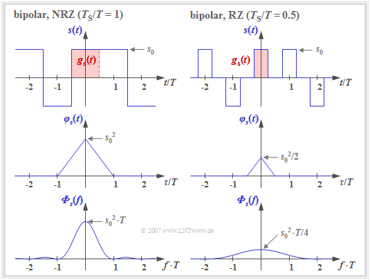
The graph shows two signal sections each with rectangular pulses $g_s(t)$, which accordingly lead to a triangular auto-correlation function $\rm (ACF)$ and to a $\rm sinc^2$–shaped power-spectral density $\rm (PSD)$.

The left pictures describe NRZ signaling ⇒ the width $T_{\rm S}$ of the basic pulse is equal to the distance $T$ of two transmitted pulses (source symbols).
In contrast, the right pictures apply to an RZ pulse with the duty cycle $T_{\rm S}/T = 0.5$.

One can see from the left representation $\rm (NRZ)$:

For NRZ rectangular pulses, the transmit power (reference: $1 \ \rm \Omega$ resistor) is $P_{\rm S} = \varphi_s(\tau = 0) = s_0^2$.
The triangular ACF is limited to the range $|\tau| \le T_{\rm S}= T$.
The PSD ${\it \Phi}_s(f)$ as the Fourier transform of $\varphi_s(\tau)$ is $\rm sinc^2$–shaped with equidistant zeros at distance $1/T$.
The area under the PSD curve again gives the transmit power $P_{\rm S} = s_0^2$.

In the case of RZ signaling (right column), the triangular ACF is smaller in height and width by a factor of $T_{\rm S}/T = 0.5$, resp., compared to the left image.

$\text{Conclusion:}$ If one compares the two power-spectral densities $($lower pictures$)$, one recognizes for $T_{\rm S}/T = 0.5$ $($RZ pulse$)$ compared to $T_{\rm S}/T = 1$ $($NRZ pulse$)$

a reduction in height by a factor of $4$,
a broadening by a factor of $2$.

⇒ The area $($power$)$ in the right sketch is thus half as large, since in half the time $s(t) = 0$.

ACF and PSD for unipolar binary signals

We continue to assume NRZ or RZ rectangular pulses. But let the binary amplitude coefficients now be unipolar: $a_\nu \in \{0, 1\}$. Then for the discrete ACF of the amplitude coefficients holds:

Signal section, ACF and PSD with binary unipolar signaling

$$\varphi_a(\lambda) = \left\{ \begin{array}{c} m_2 = 0.5 \\ \\ m_1^2 = 0.25 \\ \end{array} \right.\quad \begin{array}{*{1}c} {\rm{for}}\\ \\ {\rm{for}} \\ \end{array} \begin{array}{*{20}c}\lambda = 0, \\ \\ \lambda \ne 0 \hspace{0.05cm}.\\ \end{array}$$

Assumed here are equal probability amplitude coefficients ⇒ ${\rm Pr}(a_\nu =0) = {\rm Pr}(a_\nu =1) = 0.5$ with no statistical ties, so that both the "power" $m_2$ and the "linear mean" $m_1$ $($DC component$)$ are $0.5$, respectively.

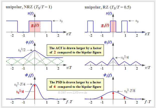
The graph shows a signal section, the ACF and the PSD with unipolar amplitude coefficients,

left for rectangular NRZ pulses $(T_{\rm S}/T = 1)$, and
right for RZ pulses with duty cycle $T_{\rm S}/T = 0.5$.

There are the following differences compared to "bipolar signaling":

Adding the infinite number of triangular functions at distance $T$ (all with the same height) results in a constant DC component $s_0^2/4$ for the ACF in the left graph (NRZ).

In addition, a single triangle also with height $s_0^2/4$ remains in the region $|\tau| \le T_{\rm S}$, which leads to the $\rm sinc^2$–shaped blue curve in the power-spectral density (PSD).

The DC component in the ACF results in a Dirac delta function at frequency $f = 0$ with weight $s_0^2/4$ in the PSD. Thus the PSD value ${\it \Phi}_s(f=0)$ becomes infinitely large.

From the right graph – valid for $T_{\rm S}/T = 0.5$ – it can be seen that now the ACF is composed of a periodic triangular function (drawn dashed in the middle region) and additionally of a unique triangle in the region $|\tau| \le T_{\rm S} = T/2$ with height $s_0^2/8$.

This unique triangle function leads to the continuous $\rm sinc^2$–shaped component (blue curve) of ${\it \Phi}_s(f)$ with the first zero at $1/T_{\rm S} = 2/T$.

In contrast, the periodic triangular function leads to an infinite sum of Dirac delta functions with different weights at the distance $1/T$ (drawn in red) according to the laws of the "Fourier series".

The weights of the Dirac delta functions are proportional to the continuous (blue) PSD component. The Dirac delta line at $f = 0$ has the maximum weight $s_0^2/8$. In contrast, the Dirac delta lines at $\pm 2/T$ and multiples thereof do not exist or have the weight $0$ in each case, since the continuous PSD component also has zeros here.

$\text{Note:}$

Unipolar amplitude coefficients occur for example in optical transmission systems.
In later chapters, however, we mostly restrict ourselves to bipolar signaling.