Difference between revisions of "Aufgaben:Exercise 3.10: Maximum Likelihood Tree Diagram"
From LNTwww
m (Guenter moved page Aufgabe 3.10: Baumdiagramm bei Maximum-Likelihood to Exercise 3.10: Maximum Likelihood Tree Diagram) |
|||
| (4 intermediate revisions by 2 users not shown) | |||
| Line 1: | Line 1: | ||
| − | {{quiz-Header|Buchseite= | + | {{quiz-Header|Buchseite=Digital_Signal_Transmission/Optimal_Receiver_Strategies}} |
| − | [[File:P_ID1465__Dig_A_3_10_95.png|right|frame| | + | [[File:P_ID1465__Dig_A_3_10_95.png|right|frame|Signals and tree diagram]] |
| − | + | As in [[Aufgaben:Exercise_3.09:_Correlation_Receiver_for_Unipolar_Signaling|"Exercise 3.9"]] we consider the joint decision of three binary symbols ("bits") by means of the correlation receiver. | |
| − | * | + | *The possible transmitted signals $s_0(t), \ \text{...} \ , \ s_7(t)$ are bipolar. |
| − | |||
| − | |||
| + | *In the graphic the functions $s_0(t)$, $s_1(t)$, $s_2(t)$ and $s_3(t)$ are shown. | ||
| − | + | *The blue curves are valid for rectangular NRZ transmission pulses. | |
| + | |||
| + | |||
| + | Below is drawn the so-called "tree diagram" for this constellation under the condition that the signal $s_3(t)$ was sent. Shown here in the range from $0$ to $3T$ are the functions | ||
:$$i_i(t) = \int_{0}^{t} s_3(\tau) \cdot s_i(\tau) \,{\rm d} | :$$i_i(t) = \int_{0}^{t} s_3(\tau) \cdot s_i(\tau) \,{\rm d} | ||
\tau \hspace{0.3cm}( i = 0, \ \text{...} \ , 7)\hspace{0.05cm}.$$ | \tau \hspace{0.3cm}( i = 0, \ \text{...} \ , 7)\hspace{0.05cm}.$$ | ||
| − | * | + | *The correlation receiver compares the final values $I_i = i_i(3T)$ with each other and searches for the largest possible value $I_j$. |
| − | * | + | |
| − | + | *The corresponding signal $s_j(t)$ is then the one most likely to have been sent according to the maximum likelihood criterion. | |
| − | |||
| − | |||
| − | |||
| − | |||
| − | |||
| − | + | *Note that the correlation receiver generally makes the decision based on the corrected quantities | |
| − | + | :$$W_i = I_i \ - E_i/2.$$ | |
| − | + | *But since for bipolar rectangles all transmitted signals $(i = 0, \ \text{...} \ , \ 7)$ have exactly the same energy | |
| + | :$$E_i = \int_{0}^{3T} s_i^2(t) \,{\rm d} t,$$ | ||
| + | :the integrals $I_i$ provide exactly the same maximum likelihood information as the corrected quantities $W_i$. | ||
| + | The red signal waveforms $s_i(t)$ are obtained from the blue ones by convolution with the impulse response $h_{\rm G}(t)$ of a Gaussian low-pass filter with cutoff frequency $f_{\rm G} \cdot T = 0.35$. | ||
| + | *Each individual rectangular pulse is broadened. | ||
| + | *The red signal waveforms lead to "intersymbol interference" in case of threshold decision. | ||
| − | + | Note: The exercise belongs to the chapter [[Digital_Signal_Transmission/Optimal_Receiver_Strategies|"Optimal Receiver Strategies"]]. | |
| − | |||
| − | |||
| − | === | + | ===Questions=== |
<quiz display=simple> | <quiz display=simple> | ||
| − | { | + | {Give the following normalized final values $I_i/E_{\rm B}$ for rectangular signals $($without noise$)$. |
|type="{}"} | |type="{}"} | ||
$I_0/E_{\rm B} \ = \ $ { -1.03--0.97 } | $I_0/E_{\rm B} \ = \ $ { -1.03--0.97 } | ||
| Line 46: | Line 46: | ||
$I_6/E_{\rm B} \ = \ $ { -1.03--0.97 } | $I_6/E_{\rm B} \ = \ $ { -1.03--0.97 } | ||
| − | { | + | {Which statements are valid when considering a noise term? |
|type="[]"} | |type="[]"} | ||
| − | - | + | - The tree diagram can be further described by straight line segments. |
| − | + | + | + If $I_3$ is the maximum $I_i$ value, the receiver decides correctly. |
| − | - | + | - $I_0 = I_6$ is valid independent of the strength of the noise. |
| − | { | + | {Which statements are valid for the red signal waveforms $($with intersymbol interference$)$? |
|type="[]"} | |type="[]"} | ||
| − | - | + | - The tree diagram can be further described by straight line segments. |
| − | + | + | + The signal energies $E_i(i = 0, \ \text{...} \ , 7$) are different. |
| − | - | + | - Both the decision variables $I_i$ and $W_i$ are suitable. |
| − | { | + | {How should the intergration range $(t_1 \ \text{...} \ t_2)$ be chosen? |
|type="[]"} | |type="[]"} | ||
| − | + | + | + Without intersymbol interference (blue), $t_1 = 0$ and $t_2 = 3T$ are best possible. |
| − | - | + | - With intersymbol interference (red), $t_1 = 0$ and $t_2 = 3T$ are best possible. |
</quiz> | </quiz> | ||
| − | === | + | ===Solution=== |
{{ML-Kopf}} | {{ML-Kopf}} | ||
| − | '''(1)''' | + | '''(1)''' The left graph shows the tree diagram (without noise) with all final values. Highlighted in green is the curve $i_0(t)/E_{\rm B}$ with the final result $I_0/E_{\rm B} = \ -1$, which first rises linearly to $+1$ $($the first bit of $s_0(t)$ and $s_3(t)$ in each case coincide$)$ and then falls off over two bit durations. |
| − | [[File: | + | [[File:EN_Dig_A_3_10_ML.png|right|frame|Tree diagram of the correlation receiver]] |
| − | + | ||
| + | *The correct results are thus: | ||
:$$I_0/E_{\rm B}\hspace{0.15cm}\underline { = -1},$$ | :$$I_0/E_{\rm B}\hspace{0.15cm}\underline { = -1},$$ | ||
:$$I_2/E_{\rm B} \hspace{0.15cm}\underline {= +1}, $$ | :$$I_2/E_{\rm B} \hspace{0.15cm}\underline {= +1}, $$ | ||
| Line 74: | Line 75: | ||
:$$I_6/E_{\rm B}\hspace{0.15cm}\underline { = -1} | :$$I_6/E_{\rm B}\hspace{0.15cm}\underline { = -1} | ||
\hspace{0.05cm}.$$ | \hspace{0.05cm}.$$ | ||
| − | |||
| − | |||
| − | |||
| − | |||
| − | |||
| − | '''(3)''' | + | '''(2)''' Only the <u>second solution</u> is correct: |
| − | * | + | *In the presence of noises, the functions $i_i(t)$ no longer increase or decrease linearly, but have a curve as shown in the right graph. |
| − | * | + | *As long as $I_3 > I_{\it i≠3}$, the correlation receiver decides correctly. |
| − | * | + | *In the presence of noise, $I_0 ≠ I_6$ always holds, in contrast to the noise-free tree diagram. |
| + | |||
| + | |||
| + | '''(3)''' Only the <u>second statement</u> is true: | ||
| + | *Since now the possible transmitted signals $s_i(t)$ can no longer be composed of isolated horizontal sections, also the tree diagram without noise does not consist of straight line segments. | ||
| + | *Since the energies $E_i$ are different – this can be seen e.g. by comparing the (red) signals $s_0(t)$ and $s_2(t)$ – it is essential to use the corrected quantities $W_i$ for the decision. | ||
| + | *The use of the uncorrected correlation values $I_i$ can already lead to wrong decisions without noise disturbances. | ||
| − | '''(4)''' | + | '''(4)''' <u>Answer 1</u> is correct: |
| − | * | + | *In the case <u>without intersymbol interference</u> (blue rectangular signals), all signals are limited to the range $0 \ ... \ 3T$. |
| − | * | + | *Outside this range the received signal $r(t)$ is pure noise. Therefore in this case also the integration over the range $0 \ \text{...} \ 3T$. |
| − | + | *In contrast, when intersymbol interference (red signals) is taken into account, the integrands $s_3(t) \cdot s_i(t)$ also differ outside this range. | |
| − | * | + | *Therefore, if $t_1 = \ -T$ and $t_2 = +4T$ are chosen, the error probability of the correlation receiver is further reduced compared to the integration range $0 \ \text{...} \ 3T$. |
| − | * | ||
{{ML-Fuß}} | {{ML-Fuß}} | ||
| Line 98: | Line 99: | ||
| − | [[Category:Digital Signal Transmission: Exercises|^3.7 | + | [[Category:Digital Signal Transmission: Exercises|^3.7 Optimal Receiver Strategies^]] |
Latest revision as of 18:24, 30 June 2022

Signals and tree diagram
As in "Exercise 3.9" we consider the joint decision of three binary symbols ("bits") by means of the correlation receiver.
- The possible transmitted signals $s_0(t), \ \text{...} \ , \ s_7(t)$ are bipolar.
- In the graphic the functions $s_0(t)$, $s_1(t)$, $s_2(t)$ and $s_3(t)$ are shown.
- The blue curves are valid for rectangular NRZ transmission pulses.
Below is drawn the so-called "tree diagram" for this constellation under the condition that the signal $s_3(t)$ was sent. Shown here in the range from $0$ to $3T$ are the functions
- $$i_i(t) = \int_{0}^{t} s_3(\tau) \cdot s_i(\tau) \,{\rm d} \tau \hspace{0.3cm}( i = 0, \ \text{...} \ , 7)\hspace{0.05cm}.$$
- The correlation receiver compares the final values $I_i = i_i(3T)$ with each other and searches for the largest possible value $I_j$.
- The corresponding signal $s_j(t)$ is then the one most likely to have been sent according to the maximum likelihood criterion.
- Note that the correlation receiver generally makes the decision based on the corrected quantities
- $$W_i = I_i \ - E_i/2.$$
- But since for bipolar rectangles all transmitted signals $(i = 0, \ \text{...} \ , \ 7)$ have exactly the same energy
- $$E_i = \int_{0}^{3T} s_i^2(t) \,{\rm d} t,$$
- the integrals $I_i$ provide exactly the same maximum likelihood information as the corrected quantities $W_i$.
The red signal waveforms $s_i(t)$ are obtained from the blue ones by convolution with the impulse response $h_{\rm G}(t)$ of a Gaussian low-pass filter with cutoff frequency $f_{\rm G} \cdot T = 0.35$.
- Each individual rectangular pulse is broadened.
- The red signal waveforms lead to "intersymbol interference" in case of threshold decision.
Note: The exercise belongs to the chapter "Optimal Receiver Strategies".
Questions
Solution
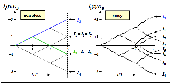
(1) The left graph shows the tree diagram (without noise) with all final values. Highlighted in green is the curve $i_0(t)/E_{\rm B}$ with the final result $I_0/E_{\rm B} = \ -1$, which first rises linearly to $+1$ $($the first bit of $s_0(t)$ and $s_3(t)$ in each case coincide$)$ and then falls off over two bit durations.

Tree diagram of the correlation receiver
- The correct results are thus:
- $$I_0/E_{\rm B}\hspace{0.15cm}\underline { = -1},$$
- $$I_2/E_{\rm B} \hspace{0.15cm}\underline {= +1}, $$
- $$I_4/E_{\rm B} \hspace{0.15cm}\underline {= -3}, $$
- $$I_6/E_{\rm B}\hspace{0.15cm}\underline { = -1} \hspace{0.05cm}.$$
(2) Only the second solution is correct:
- In the presence of noises, the functions $i_i(t)$ no longer increase or decrease linearly, but have a curve as shown in the right graph.
- As long as $I_3 > I_{\it i≠3}$, the correlation receiver decides correctly.
- In the presence of noise, $I_0 ≠ I_6$ always holds, in contrast to the noise-free tree diagram.
(3) Only the second statement is true:
- Since now the possible transmitted signals $s_i(t)$ can no longer be composed of isolated horizontal sections, also the tree diagram without noise does not consist of straight line segments.
- Since the energies $E_i$ are different – this can be seen e.g. by comparing the (red) signals $s_0(t)$ and $s_2(t)$ – it is essential to use the corrected quantities $W_i$ for the decision.
- The use of the uncorrected correlation values $I_i$ can already lead to wrong decisions without noise disturbances.
(4) Answer 1 is correct:
- In the case without intersymbol interference (blue rectangular signals), all signals are limited to the range $0 \ ... \ 3T$.
- Outside this range the received signal $r(t)$ is pure noise. Therefore in this case also the integration over the range $0 \ \text{...} \ 3T$.
- In contrast, when intersymbol interference (red signals) is taken into account, the integrands $s_3(t) \cdot s_i(t)$ also differ outside this range.
- Therefore, if $t_1 = \ -T$ and $t_2 = +4T$ are chosen, the error probability of the correlation receiver is further reduced compared to the integration range $0 \ \text{...} \ 3T$.