Difference between revisions of "Aufgaben:Exercise 3.2Z: Relationship between PDF and CDF"
From LNTwww
m (Nabil verschob die Seite Zusatzaufgaben:3.2 Zusammenhang WDF/VTF nach 3.2Z Zusammenhang WDF/VTF) |
|||
| (22 intermediate revisions by 4 users not shown) | |||
| Line 1: | Line 1: | ||
| − | {{quiz-Header|Buchseite= | + | {{quiz-Header|Buchseite=Theory_of_Stochastic_Signals/Cumulative_Distribution_Function |
}} | }} | ||
| − | [[File:P_ID117__Sto_Z_3_2.png|right|]] | + | [[File:P_ID117__Sto_Z_3_2.png|right|frame|Given CDF $ F_x(r)$]] |
| − | + | Given is the random variable $x$ with the cumulative distribution function $\rm (CDF)$. | |
| − | :$$ F_x(r)=\left\{\begin{array}{*{4}{c}} 0.25\cdot {\rm e}^{2\it r} &\rm | + | :$$ F_x(r)=\left\{\begin{array}{*{4}{c}} 0.25\cdot {\rm e}^{2\it r} &\rm for\hspace{0.1cm}\it r<\rm 0, \\ 1-0.25\cdot {\rm e}^{-2\it r} & \rm for\hspace{0.1cm}\it r\ge\rm 0. \\\end{array}\right.$$ |
| − | + | *This function is shown on the right. | |
| + | *It can be seen that at the unit step point $r = 0$ the right-hand side limit is valid. | ||
| − | |||
| − | |||
| − | |||
| − | === | + | |
| + | |||
| + | Hints: | ||
| + | *The exercise belongs to the chapter [[Theory_of_Stochastic_Signals/Cumulative_Distribution_Function|Cumulative Distribution Function]]. | ||
| + | *Reference is made to the chapter [[Theory_of_Stochastic_Signals/Probability_Density_Function|Probability Density Function]]. | ||
| + | *The topic of this chapter is illustrated with examples in the (German language) learning video <br> [[Zusammenhang_zwischen_WDF_und_VTF_(Lernvideo)|"Zusammenhang zwischen WDF und VTF"]] $\Rightarrow$ "Relationship between PDF and CDF". | ||
| + | |||
| + | |||
| + | |||
| + | |||
| + | |||
| + | ===Questions=== | ||
<quiz display=simple> | <quiz display=simple> | ||
| − | { | + | {What properties of the CDF hold when the random variable has no limits? |
|type="[]"} | |type="[]"} | ||
| − | + | + | + The CDF increases from $0$ to $1$ at least weakly monotonically. |
| − | - | + | - The $F_x(r)$ values $0$ and $1$ are possible for finite $r$ values. |
| − | + | + | +A horizontal section indicates that in this range the random size has no proportions. |
| − | + | + | +Vertical sections are possible. |
| − | { | + | {What is the probability that $x$ is positive? |
|type="{}"} | |type="{}"} | ||
| − | $Pr(x > 0)$ | + | ${\rm Pr}(x > 0) \ = \ $ { 0.25 3% } |
| − | { | + | {What is the probability that $|\hspace{0.05cm}x\hspace{0.05cm}|$ is larger than $0.5$? |
|type="{}"} | |type="{}"} | ||
| − | $Pr (|x| > 0.5)$ | + | ${\rm Pr}(|\hspace{0.05cm}x\hspace{0.05cm}| > 0.5) \ = \ $ { 0.184 3% } |
| − | { | + | {Specify the associated PDF $f_x(x)$ in general and the value for $x = 1$. |
|type="{}"} | |type="{}"} | ||
| − | $f_x(x\ =\ | + | $f_x(x =1)\ = \ $ { 0.0677 3% } |
| − | { | + | {What is the probability that $x$ is exactly equal to $1$ ? |
|type="{}"} | |type="{}"} | ||
| − | $Pr(x = 1)$ | + | ${\rm Pr}(x = 1)\ = \ $ { 0. } |
| − | { | + | {What is the probability that $x$ is exactly equal to $0$ ? |
|type="{}"} | |type="{}"} | ||
| − | $Pr(x = 0)$ | + | ${\rm Pr}(x = 0)\ = \ $ { 0.5 3% } |
| − | |||
</quiz> | </quiz> | ||
| − | === | + | ===Solution=== |
{{ML-Kopf}} | {{ML-Kopf}} | ||
| − | + | '''(1)''' The <u>statements 1, 3 and 4</u> are always correct: | |
| + | *A horizontal intercept in the CDF indicates that the random variable has no values in that region. | ||
| + | *In contrast, a vertical intercept in the CDF indicates a Dirac delta function in the PDF $($at the same location $x_0)$. | ||
| + | *This means that the random variable takes the value $x_0$ very frequently, namely with finite probability. | ||
| + | *All other values occur exactly with probability $0$. | ||
| + | *If, however $x$ is limited to the range from $x_{\rm min}$ to $x_{\rm max}$ then $F_x(r) = 0$ for $r < x_{\rm min}$ and $F_x(r) = 1$ for $r > x_{\rm max}$. | ||
| + | *In this special case, the second statement would also be true. | ||
| + | |||
| − | |||
| − | + | '''(2)''' The sought probability can be calculated from the difference of the CDF values at the boundaries: | |
| − | :$$\rm Pr( | + | :$${\rm Pr}( x> 0)= F_x(\infty)- F_x(\rm 0) |
\hspace{0.15cm}\underline{=\rm 0.25}.$$ | \hspace{0.15cm}\underline{=\rm 0.25}.$$ | ||
| − | + | ||
| − | :$$\rm Pr( | + | |
| + | '''(3)''' For the probability that $x$ is greater than $0.5$ holds: | ||
| + | :$${\rm Pr}(x> 0.5)=1- F_x(0.5)=\rm 0.25\cdot e^{-1} | ||
\hspace{0.15cm}{\approx0.092}. $$ | \hspace{0.15cm}{\approx0.092}. $$ | ||
| − | : | + | *For reasons of symmetry: ${\rm Pr}(x<- 0.5)$ is just as large. From this follows: |
| − | :$$\rm Pr( |\ | + | :$${\rm Pr}( |\hspace{0.05cm} x\hspace{0.05cm}| >\rm 0.5) \hspace{0.15cm}\underline{= \rm 0.184}.$$ |
| + | |||
| + | |||
| + | [[File: P_ID116__Sto_Z_3_2_c.png|right|frame|PDF of Laplace distribution]] | ||
| + | '''(4)''' The PDF is obtained from the corresponding CDF by differentiating the two areas. | ||
| + | *The result is a two-sided exponential function as well as a Dirac delta function at $x = 0$: | ||
| + | :$$f_x(x)=\rm 0.5\cdot \rm e^{-2\cdot |\hspace{0.05cm}\it x\hspace{0.05cm}|} + \rm 0.5\cdot\delta(\it x).$$ | ||
| + | *The numerical value we are looking for is $f_x(x = 1)\hspace{0.15cm}\underline{= \rm 0.0677}$. | ||
| + | *Note: The two-sided exponential distribution is also called "Laplace distribution". | ||
| + | |||
| + | |||
| − | + | '''(5)''' In the range around $1$ describes $x$ a continuous valued random variable. | |
| − | + | *The probability that $x$ has exactly the value $1$ is therefore ${\rm Pr}(x = 1)\hspace{0.15cm}\underline{= \rm 0}.$ | |
| − | |||
| − | |||
| − | |||
| − | + | '''(6)''' In $50\%$ of time $x = 0$ will hold: ${\rm Pr}(x = 0)\hspace{0.15cm}\underline{= \rm 0.5}.$ | |
| − | + | *The PDF of a speech signal is often described by a two-sided exponential function. | |
| + | *The Dirac delta function at $x = 0$ mainly takes into account speech pauses – here in $50\%$ of all times. | ||
{{ML-Fuß}} | {{ML-Fuß}} | ||
| − | [[Category: | + | [[Category:Theory of Stochastic Signals: Exercises|^3.2 Cumulative Distribution Function^]] |
Latest revision as of 16:39, 4 January 2022

Given CDF $ F_x(r)$
Given is the random variable $x$ with the cumulative distribution function $\rm (CDF)$.
- $$ F_x(r)=\left\{\begin{array}{*{4}{c}} 0.25\cdot {\rm e}^{2\it r} &\rm for\hspace{0.1cm}\it r<\rm 0, \\ 1-0.25\cdot {\rm e}^{-2\it r} & \rm for\hspace{0.1cm}\it r\ge\rm 0. \\\end{array}\right.$$
- This function is shown on the right.
- It can be seen that at the unit step point $r = 0$ the right-hand side limit is valid.
Hints:
- The exercise belongs to the chapter Cumulative Distribution Function.
- Reference is made to the chapter Probability Density Function.
- The topic of this chapter is illustrated with examples in the (German language) learning video
"Zusammenhang zwischen WDF und VTF" $\Rightarrow$ "Relationship between PDF and CDF".
Questions
Solution
(1) The statements 1, 3 and 4 are always correct:
- A horizontal intercept in the CDF indicates that the random variable has no values in that region.
- In contrast, a vertical intercept in the CDF indicates a Dirac delta function in the PDF $($at the same location $x_0)$.
- This means that the random variable takes the value $x_0$ very frequently, namely with finite probability.
- All other values occur exactly with probability $0$.
- If, however $x$ is limited to the range from $x_{\rm min}$ to $x_{\rm max}$ then $F_x(r) = 0$ for $r < x_{\rm min}$ and $F_x(r) = 1$ for $r > x_{\rm max}$.
- In this special case, the second statement would also be true.
(2) The sought probability can be calculated from the difference of the CDF values at the boundaries:
- $${\rm Pr}( x> 0)= F_x(\infty)- F_x(\rm 0) \hspace{0.15cm}\underline{=\rm 0.25}.$$
(3) For the probability that $x$ is greater than $0.5$ holds:
- $${\rm Pr}(x> 0.5)=1- F_x(0.5)=\rm 0.25\cdot e^{-1} \hspace{0.15cm}{\approx0.092}. $$
- For reasons of symmetry: ${\rm Pr}(x<- 0.5)$ is just as large. From this follows:
- $${\rm Pr}( |\hspace{0.05cm} x\hspace{0.05cm}| >\rm 0.5) \hspace{0.15cm}\underline{= \rm 0.184}.$$

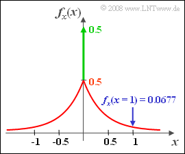
PDF of Laplace distribution
(4) The PDF is obtained from the corresponding CDF by differentiating the two areas.
- The result is a two-sided exponential function as well as a Dirac delta function at $x = 0$:
- $$f_x(x)=\rm 0.5\cdot \rm e^{-2\cdot |\hspace{0.05cm}\it x\hspace{0.05cm}|} + \rm 0.5\cdot\delta(\it x).$$
- The numerical value we are looking for is $f_x(x = 1)\hspace{0.15cm}\underline{= \rm 0.0677}$.
- Note: The two-sided exponential distribution is also called "Laplace distribution".
(5) In the range around $1$ describes $x$ a continuous valued random variable.
- The probability that $x$ has exactly the value $1$ is therefore ${\rm Pr}(x = 1)\hspace{0.15cm}\underline{= \rm 0}.$
(6) In $50\%$ of time $x = 0$ will hold: ${\rm Pr}(x = 0)\hspace{0.15cm}\underline{= \rm 0.5}.$
- The PDF of a speech signal is often described by a two-sided exponential function.
- The Dirac delta function at $x = 0$ mainly takes into account speech pauses – here in $50\%$ of all times.