Difference between revisions of "Aufgaben:Exercise 4.12: Calculations for the 16-QAM"
From LNTwww
| Line 1: | Line 1: | ||
| − | {{quiz-Header|Buchseite= | + | {{quiz-Header|Buchseite=Digital_Signal_Transmission/Carrier_Frequency_Systems_with_Coherent_Demodulation}} |
| − | [[File:P_ID2062__Dig_A_4_12.png|right|frame| | + | [[File:P_ID2062__Dig_A_4_12.png|right|frame|Signal space constellation of 16–QAM]] |
| − | + | The graphic shows the signal space constellation of the [[Digital_Signal_Transmission/Carrier_Frequency_Systems_with_Coherent_Demodulation#Quadrature_amplitude_modulation_.28M-QAM.29|"quadrature amplitude modulation"]] with $M = 16$ signal space points. | |
| − | + | The following should be calculated for this modulation method: | |
| − | * | + | * the average energy per symbol or per bit, |
| − | * | + | * the mean symbol error probability $p_{\rm S}$, |
| − | * | + | *the [[Digital_Signal_Transmission/Approximation_of_the_Error_Probability#Union_Bound_-_Upper_bound_for_the_error_probability|"Union Bound"]] $p_{\rm UB}$ as upper bound, |
| − | * | + | * the average bit error probability $p_{\rm B}$ with Gray coding. |
| Line 15: | Line 15: | ||
| − | '' | + | ''Notes:'' |
| − | * | + | * The exercise deals with a partial aspect of the chapter [[Digital_Signal_Transmission/Carrier_Frequency_Systems_with_Coherent_Demodulation|"Carrier Frequency Systems with Coherent Demodulation]]. |
| − | * | + | *The Gray assignment is given in the graphic (red lettering). |
| − | * | + | * The probability that the upper left symbol is falsified into one of the neighboring symbols is abbreviated to $p$ (blue arrows in the graph). |
| − | * | + | * A diagonal falsification ⇒ two bit falsified (green arrow) is excluded. |
| − | * | + | * For the AWGN channel, with the complementary Gaussian error integral for this auxiliary variable, the following applies: $p = {\rm Q} \left ( \sqrt{ { 2E}/{ N_0} }\right )\hspace{0.05cm}.$ |
| − | * | + | * For numerical calculations, use $E = 1 \ \rm mWs$ and $p = 0.4\%$. |
| − | * | + | *The AWGN noise power density $N_0$ can be calculated approximately from these values: |
:$$p = {\rm Q} \left ( \sqrt{ { 2E}/{ N_0} }\right ) = 0.004 \hspace{0.1cm}\Rightarrow\hspace{0.1cm} | :$$p = {\rm Q} \left ( \sqrt{ { 2E}/{ N_0} }\right ) = 0.004 \hspace{0.1cm}\Rightarrow\hspace{0.1cm} | ||
{ 2E}{ N_0} \approx 2.65^2 \approx 7 \hspace{0.1cm}\Rightarrow\hspace{0.1cm} N_0 = { E}/{ 3.5}\approx 1.4 \cdot 10^{-4}\,{\rm W/Hz} | { 2E}{ N_0} \approx 2.65^2 \approx 7 \hspace{0.1cm}\Rightarrow\hspace{0.1cm} N_0 = { E}/{ 3.5}\approx 1.4 \cdot 10^{-4}\,{\rm W/Hz} | ||
| Line 30: | Line 30: | ||
| − | === | + | ===Questions=== |
<quiz display=simple> | <quiz display=simple> | ||
| − | { | + | {Let $E = 1 \ \rm mWs$. What is the average energy ''per symbol''? |
|type="{}"} | |type="{}"} | ||
$E_{\rm S}\ = \ $ { 10 3% } $\ \rm mWs$ | $E_{\rm S}\ = \ $ { 10 3% } $\ \rm mWs$ | ||
Revision as of 16:14, 19 July 2022

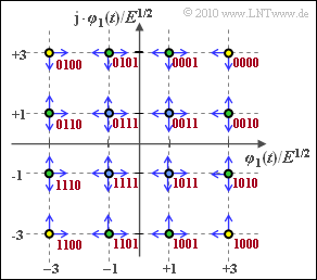
Signal space constellation of 16–QAM
The graphic shows the signal space constellation of the "quadrature amplitude modulation" with $M = 16$ signal space points.
The following should be calculated for this modulation method:
- the average energy per symbol or per bit,
- the mean symbol error probability $p_{\rm S}$,
- the "Union Bound" $p_{\rm UB}$ as upper bound,
- the average bit error probability $p_{\rm B}$ with Gray coding.
Notes:
- The exercise deals with a partial aspect of the chapter "Carrier Frequency Systems with Coherent Demodulation.
- The Gray assignment is given in the graphic (red lettering).
- The probability that the upper left symbol is falsified into one of the neighboring symbols is abbreviated to $p$ (blue arrows in the graph).
- A diagonal falsification ⇒ two bit falsified (green arrow) is excluded.
- For the AWGN channel, with the complementary Gaussian error integral for this auxiliary variable, the following applies: $p = {\rm Q} \left ( \sqrt{ { 2E}/{ N_0} }\right )\hspace{0.05cm}.$
- For numerical calculations, use $E = 1 \ \rm mWs$ and $p = 0.4\%$.
- The AWGN noise power density $N_0$ can be calculated approximately from these values:
- $$p = {\rm Q} \left ( \sqrt{ { 2E}/{ N_0} }\right ) = 0.004 \hspace{0.1cm}\Rightarrow\hspace{0.1cm} { 2E}{ N_0} \approx 2.65^2 \approx 7 \hspace{0.1cm}\Rightarrow\hspace{0.1cm} N_0 = { E}/{ 3.5}\approx 1.4 \cdot 10^{-4}\,{\rm W/Hz} \hspace{0.05cm}.$$
Questions
Musterlösung
(1) Der Quotient $E_{\rm S}/E$ ergibt sich als der mittlere quadratische Abstand der $M = 16$ Signalraumpunkte $\boldsymbol{s}_i$ vom Ursprung.
- Mit der gegebenen Signalraumkonstellation der 16–QAM erhält man:
- $$E_{\rm S} \hspace{-0.1cm} \ = \ \hspace{-0.1cm} { E}/{ 16} \cdot \left [ 4 \cdot (1^2 + 1^2) + 8 \cdot (1^2 + 3^2) + 4 \cdot (3^2 + 3^2)\right ]={ E}/{ 16} \cdot \left [ 4 \cdot 2 + 8 \cdot 10 + 4 \cdot 18\right ] = 10 \cdot E = \underline{10 \ {\rm mWs}} \hspace{0.05cm}.$$
- Zum gleichen Ergebnis kommt man mit der im Theorieteil angegebenen Gleichung
- $$E_{\rm S} = \frac{ 2 \cdot (M-1)}{ 3 } \cdot E = \frac{ 2 \cdot 15}{ 3 } \cdot E = 10 E \hspace{0.05cm}.$$
(2) Jedes einzelne Symbol stellt vier Binärsymbole dar. Damit ist die mittlere Energie pro Bit.
- $$E_{\rm B} = \frac{ E_{\rm S}}{ {\rm log_2} \hspace{0.05cm}(M)} = 2.5 \cdot E = \underline{2.5 \ {\rm mWs}} \hspace{0.05cm}.$$

Zur Verdeutlichung der 16–QAM–Fehlerwahrscheinlichkeit
(3) Die Union Bound ist eine obere Schranke für die Symbolfehlerwahrscheinlichkeit.
- Sie berücksichtigt nur den Übergang zu benachbarten Entscheidungsregionen aufgrund von AWGN–Rauschen.
- Aus der Grafik geht hervor, dass die Ecksymbole (gelb gefüllt) nur zu zwei anderen Symbolen hin verfälscht werden können und die restlichen Randsymbole (grüne Füllung) in drei Richtungen.
- Der "worst case" sind die vier inneren Symbole (mit blauer Füllung) mit jeweils vier Verfälschungsmöglichkeiten. Daraus folgt:
- $$p_{\rm S} = {\rm Pr}({\cal{E}}) \le 4 \cdot p = \underline{1.6\%}= p_{\rm UB} \hspace{0.05cm}.$$
(4) Zählt man die blauen Pfeile in obiger Grafik, so kommt man auf
- $$4 \cdot 2 + 8 \cdot 3 + 4 \cdot 4 = 48.$$
- Die mittlere Symbolfehlerwahrscheinlichkeit ist somit gleich
- $$p_{\rm S} = { E}/{ 16} \cdot 48 p = 3p = \underline{1.2\%} \hspace{0.05cm}.$$
- Zum gleichen Ergebnis kommt man mit der im Theorieteil angegebenen Gleichung
- $$p_{\rm S} = 4p \cdot \left [ 1 - { 1}/{ \sqrt{M}} \right ] = 4p \cdot \left [ 1 - { 1}/{ 4} \right ] = 3p \hspace{0.05cm}.$$
- Beide Gleichungen gelten nur dann exakt, wenn man wie hier diagonale Verfälschungen ausschließt.
(5) Bei Graycodierung entsprechend der roten Beschriftung in der Grafik bewirkt jeder Symbolfehler genau einen Bitfehler.
- Da aber mit jedem Symbol $M = 4$ Binärsymbole übertragen werden, ist
- $$p_{\rm B} = \frac{ p_{\rm S}}{ {\rm log_2} \hspace{0.05cm}(M)} = \frac{ 1.2\%}{ 4} = \underline{0.3\%} \hspace{0.05cm}.$$