Difference between revisions of "Aufgaben:Exercise 5.2: Band Spreading and Narrowband Interferer"
From LNTwww
m (Text replacement - "„" to """) |
m (Text replacement - "power spectral density" to "power-spectral density") |
||
| (13 intermediate revisions by 3 users not shown) | |||
| Line 1: | Line 1: | ||
| − | {{quiz-Header|Buchseite= | + | {{quiz-Header|Buchseite=Modulation_Methods/Direct-Sequence_Spread_Spectrum_Modulation |
}} | }} | ||
| − | [[File: | + | [[File:EN_Mod_A_5_2.png|right|frame|Considered model<br> |
| − | + | of band spreading]] | |
| − | * | + | A spread spectrum system is considered according to the given diagram in the equivalent low-pass range: |
| + | *Let the digital signal $q(t)$ possess the power-spectral density ${\it \Phi}_q(f)$, which is to be approximated as rectangular with bandwidth $B = 1/T = 100\ \rm kHz$ (a rather unrealistic assumption): | ||
:$${\it \Phi}_{q}(f) = | :$${\it \Phi}_{q}(f) = | ||
| − | \left\{ \begin{array}{c} {\it \Phi}_{ | + | \left\{ \begin{array}{c} {\it \Phi}_{0} \\ |
0 \\ \end{array} \right. | 0 \\ \end{array} \right. | ||
| − | \begin{array}{*{10}c} {\rm{ | + | \begin{array}{*{10}c} {\rm{for}} |
| − | \\ {\rm{ | + | \\ {\rm{otherwise}} \hspace{0.05cm}. \\ \end{array}\begin{array}{*{20}c} |
|f| <B/2 \hspace{0.05cm}, \\ | |f| <B/2 \hspace{0.05cm}, \\ | ||
\\ | \\ | ||
\end{array}$$ | \end{array}$$ | ||
| − | * | + | *Thus, in the low-pass range, the bandwidth (only the components at positive frequencies) is equal to $B/2$ and the bandwidth in the band-pass range is $B$. |
| − | * | + | *The band spreading is done by multiplication with the PN sequence $c(t)$ of the chip duration $T_c = T/100$ <br>("PN" stands for "pseudo-noise"). |
| − | * | + | *To simplify matters, the following applies to the auto-correlation function: |
| − | :$$ {\it \varphi}_{c}(\tau) = \left\{ \begin{array}{c}1 - |\tau|/T_c \\ 0 \\ \end{array} \right. \begin{array}{*{10}c} {\rm{ | + | :$$ {\it \varphi}_{c}(\tau) = \left\{ \begin{array}{c}1 - |\tau|/T_c \\ 0 \\ \end{array} \right. \begin{array}{*{10}c} {\rm{for}} \\ {\rm{otherwise}} \hspace{0.05cm}. \\ \end{array}\begin{array}{*{20}c} -T_c \le \tau \le T_c \hspace{0.05cm}, \\ \\ \end{array}$$ |
| − | * | + | *At the receiver, the same spreading sequence $c(t)$ is again added phase-synchronously. |
| − | * | + | *The interference signal $i(t)$ is to be neglected for the time being. |
| − | *In | + | *In subtask '''(4)''' $i(t)$ denotes a narrowband interferer at carrier frequency $f_{\rm T} = 30 \ \rm MHz = f_{\rm I}$ with power $P_{\rm I}$. |
| − | * | + | *The influence of the (always present) AWGN noise $n(t)$ is not considered in this exercise. |
| − | + | Note: | |
| − | + | *This exercise belongs to the chapter [[Modulation_Methods/PN–Modulation|Direct-Sequence Spread Spectrum Modulation]]. | |
| − | |||
| − | |||
| − | |||
| − | * | ||
| − | === | + | ===Questions=== |
<quiz display=simple> | <quiz display=simple> | ||
| − | { | + | {What is the power-spectral density ${\it \Phi}_c(f )$ of the spreading signal $c(t)$? What value results at the frequency $f = 0$? |
|type="{}"} | |type="{}"} | ||
${\it \Phi}_c(f = 0) \ = \ $ { 0.1 3% } $\ \cdot 10^{-6} \ \rm 1/Hz$ | ${\it \Phi}_c(f = 0) \ = \ $ { 0.1 3% } $\ \cdot 10^{-6} \ \rm 1/Hz$ | ||
| − | { | + | {Calculate the equivalent bandwidth $B_c$ of the spread signal as the width of the equal-area $\rm PDS$ rectangle. |
|type="{}"} | |type="{}"} | ||
$B_c \ = \ $ { 10 3% } $\ \rm MHz$ | $B_c \ = \ $ { 10 3% } $\ \rm MHz$ | ||
| − | { | + | {Which statements are true for the bandwidths of the signals $s(t)$ ⇒ $B_s$ and $b(t)$ ⇒ $B_b$? The (two-sided) bandwidth of $q(t)$ is $B$. |
|type="[]"} | |type="[]"} | ||
| − | - $B_s$ | + | - $B_s$ is exactly equal to $B_c$. |
| − | + $B_s$ | + | + $B_s$ is approximately equal to $B_c + B$. |
| − | - $B_b$ | + | - $B_b$ is exactly equal to $B_s$. |
| − | - $B_b$ | + | - $B_b$ is equal to $B_s + B_c = 2B_c + B$. |
| − | + $B_b$ | + | + $B_b$ is exactly equal to $B$. |
| − | { | + | {What is the effect of band spreading on a "narrowband interferer" at the carrier frequency? Let $f_{\rm I} = f_{\rm T}$. |
|type="[]"} | |type="[]"} | ||
| − | + | + | + The interfering influence is weakened by band spreading. |
| − | - | + | - The interfering power is only half as large. |
| − | - | + | - The interfering power is not changed by band spreading. |
</quiz> | </quiz> | ||
| − | === | + | ===Solution=== |
{{ML-Kopf}} | {{ML-Kopf}} | ||
| − | '''(1)''' | + | '''(1)''' The power-spectral density $\rm (PDS)$ ${\it \Phi}_c(f)$ is the Fourier transform of the triangular ACF, which can be represented with rectangles of width $T_c$ as follows: |
:$${\it \varphi}_{c}(\tau) = \frac{1}{T_c} \cdot {\rm rect} \big(\frac{\tau}{T_c} \big ) \star {\rm rect} \big(\frac{\tau}{T_c} \big ) \hspace{0.05cm}.$$ | :$${\it \varphi}_{c}(\tau) = \frac{1}{T_c} \cdot {\rm rect} \big(\frac{\tau}{T_c} \big ) \star {\rm rect} \big(\frac{\tau}{T_c} \big ) \hspace{0.05cm}.$$ | ||
| − | * | + | *From this follows ${\it \Phi}_{c}(f) = {1}/{T_c} \cdot \big[ T_c \cdot {\rm sinc} \left(f T_c \right ) \big ] \cdot \big[ T_c \cdot {\rm sinc} \left(f T_c \right ) \big ] = T_c \cdot {\rm sinc}^2 \left(f T_c \right ) \hspace{0.05cm}$ with maximum value |
:$${\it \Phi}_{c}(f = 0) = T_c = \frac{T}{100}= \frac{1}{100 \cdot B} = \frac{1}{100 \cdot 10^5\,{\rm 1/s}} = 10^{-7}\,{\rm 1/Hz} \hspace{0.15cm}\underline {= 0.1 \cdot 10^{-6}\,{\rm 1/Hz}}\hspace{0.05cm}.$$ | :$${\it \Phi}_{c}(f = 0) = T_c = \frac{T}{100}= \frac{1}{100 \cdot B} = \frac{1}{100 \cdot 10^5\,{\rm 1/s}} = 10^{-7}\,{\rm 1/Hz} \hspace{0.15cm}\underline {= 0.1 \cdot 10^{-6}\,{\rm 1/Hz}}\hspace{0.05cm}.$$ | ||
| − | + | '''(2)''' By definition, with $T_c = T/100 = 0.1\ \rm µ s$: | |
| − | + | [[File:P_ID1869__Mod_A_5_2b.png|right|frame|Power density spectrum of the pseudo-noise spread signal]] | |
| − | + | :$$B_c= \frac{1}{T_c} \cdot \hspace{-0.03cm} \int_{-\infty }^{+\infty} \hspace{-0.03cm} {\it \Phi}_{c}(f)\hspace{0.1cm} {\rm d}f = \hspace{-0.03cm} \int_{-\infty }^{+\infty} \hspace{-0.03cm} {\rm sinc}^2 \left(f T_c \right )\hspace{0.1cm} {\rm d}f $$ | |
| − | '''(2)''' | + | :$$\Rightarrow \hspace{0.3cm} B_c= \frac{1}{T_c}\hspace{0.15cm}\underline {= 10\,{\rm MHz}} \hspace{0.05cm}$$ |
| − | :$$B_c= \frac{1}{T_c} \cdot \hspace{-0.03cm} \int_{-\infty }^{+\infty} \hspace{-0.03cm} {\it \Phi}_{c}(f)\hspace{0.1cm} {\rm d}f = \hspace{-0.03cm} \int_{-\infty }^{+\infty} \hspace{-0.03cm} {\rm | + | The graph illustrates, |
| − | :$$\Rightarrow \hspace{0.3cm} B_c= | + | *that $B_c$ is given by the first zero of the $\rm sinc^2$ function in the equivalent low-pass range, |
| − | + | *but at the same time also gives the equivalent (equal area) bandwidth in the band-pass region. | |
| − | * | ||
| − | * | ||
| − | |||
| − | '''(3)''' | + | '''(3)''' <u>Solutions 2 and 5</u> are correct: |
| − | * | + | *The PDS ${\it \Phi}_s(f)$ results from the convolution of ${\it \Phi}_q(f)$ and ${\it \Phi}_c(f)$. This actually gives $B_s = B_c + B$ for the bandwidth of the transmitted signal. |
| − | * | + | *Since the spreading signal $c(t) ∈ \{+1, –1\}$ multiplied by itself always gives the value $1$, naturally $b(t) ≡ q(t)$ and consequently $B_b = B$. |
| − | * | + | *Obviously, the bandwidth $B_b$ of the band compressed signal is not equal to $2B_c + B$, although the convolution ${\it \Phi}_s(f) ∗ {\it \Phi}_c(f)$ suggests this. |
| − | * | + | *This is due to the fact that the power density spectra must not be convolved, but the spectral functions (amplitude spectra) $S(f)$ and $C(f)$ must be assumed, taking into account the phase relations. |
| − | * | + | *Only then can the PDS $B(f)$ be determined from ${\it \Phi}_b(f)$. Clearly, the following is also true: $C(f) ∗ C(f) = δ(f)$. |
| − | '''(4)''' | + | '''(4)''' Only the <u>first solution</u> is correct. The solution shall be clarified by the diagram at the end of the page: |
| − | * | + | *In the upper diagram the PDS ${\it \Phi}_i(f)$ of the narrowband interferer is approximated by two Dirac delta functions at $±f_{\rm T}$ with weights $P_{\rm I}/2$. Also plotted is the bandwidth $B = 0.1 \ \rm MHz$ (not quite true to scale). |
| − | * | + | *The receiver-side multiplication with $c(t)$ – actually with the function of the band compression, at least with respect to the useful part of $r(t)$ – causes a band spreading with respect to the interference signal $i(t)$. Without considering the useful signal, $b(t) = n(t) = i(t) · c(t)$. It follows: |
| − | :$${\it \Phi}_{n}(f) = {\it \Phi}_{i}(f) \star {\it \Phi}_{c}(f) = \frac{P_{\rm I}\cdot T_c}{2}\cdot {\rm | + | :$${\it \Phi}_{n}(f) = {\it \Phi}_{i}(f) \star {\it \Phi}_{c}(f) = \frac{P_{\rm I}\cdot T_c}{2}\cdot {\rm sinc}^2 \left( (f - f_{\rm T}) \cdot T_c \right )+ \frac{P_{\rm I}\cdot T_c}{2}\cdot {\rm sinc}^2 \left( (f + f_{\rm T}) \cdot T_c \right ) \hspace{0.05cm}.$$ |
| − | [[File:P_ID1870__Mod_A_5_2c.png|right|frame| | + | [[File:P_ID1870__Mod_A_5_2c.png|right|frame|Power density spectra before and after band spreading]] |
| − | * | + | *Note that $n(t)$ is used here only as an abbreviation and does not denote AWGN noise. |
| − | *In | + | *In a narrow range around the carrier frequency $f_{\rm T} = 30 \ \rm MHz$, the PDS ${\it \Phi}_n(f)$ is almost constant. Thus, the interference power after band spreading is: |
:$$ P_{n} = P_{\rm I} \cdot T_c \cdot B = P_{\rm I}\cdot \frac{B}{B_c} = \frac{P_{\rm I}}{J}\hspace{0.05cm}. $$ | :$$ P_{n} = P_{\rm I} \cdot T_c \cdot B = P_{\rm I}\cdot \frac{B}{B_c} = \frac{P_{\rm I}}{J}\hspace{0.05cm}. $$ | ||
| − | * | + | *This means: The interference power is reduced by the factor $J = T/T_c$ by band spreading, which is why $J$ is often called "spreading gain". |
| − | * | + | *However, such a "spreading gain" is only given for a narrowband interferer. |
| Line 108: | Line 102: | ||
| − | [[Category:Modulation Methods: Exercises|^5.2 | + | [[Category:Modulation Methods: Exercises|^5.2 PN Modulation^]] |
Latest revision as of 13:41, 17 February 2022

Considered model
of band spreading
of band spreading
A spread spectrum system is considered according to the given diagram in the equivalent low-pass range:
- Let the digital signal $q(t)$ possess the power-spectral density ${\it \Phi}_q(f)$, which is to be approximated as rectangular with bandwidth $B = 1/T = 100\ \rm kHz$ (a rather unrealistic assumption):
- $${\it \Phi}_{q}(f) = \left\{ \begin{array}{c} {\it \Phi}_{0} \\ 0 \\ \end{array} \right. \begin{array}{*{10}c} {\rm{for}} \\ {\rm{otherwise}} \hspace{0.05cm}. \\ \end{array}\begin{array}{*{20}c} |f| <B/2 \hspace{0.05cm}, \\ \\ \end{array}$$
- Thus, in the low-pass range, the bandwidth (only the components at positive frequencies) is equal to $B/2$ and the bandwidth in the band-pass range is $B$.
- The band spreading is done by multiplication with the PN sequence $c(t)$ of the chip duration $T_c = T/100$
("PN" stands for "pseudo-noise"). - To simplify matters, the following applies to the auto-correlation function:
- $$ {\it \varphi}_{c}(\tau) = \left\{ \begin{array}{c}1 - |\tau|/T_c \\ 0 \\ \end{array} \right. \begin{array}{*{10}c} {\rm{for}} \\ {\rm{otherwise}} \hspace{0.05cm}. \\ \end{array}\begin{array}{*{20}c} -T_c \le \tau \le T_c \hspace{0.05cm}, \\ \\ \end{array}$$
- At the receiver, the same spreading sequence $c(t)$ is again added phase-synchronously.
- The interference signal $i(t)$ is to be neglected for the time being.
- In subtask (4) $i(t)$ denotes a narrowband interferer at carrier frequency $f_{\rm T} = 30 \ \rm MHz = f_{\rm I}$ with power $P_{\rm I}$.
- The influence of the (always present) AWGN noise $n(t)$ is not considered in this exercise.
Note:
- This exercise belongs to the chapter Direct-Sequence Spread Spectrum Modulation.
Questions
Solution
(1) The power-spectral density $\rm (PDS)$ ${\it \Phi}_c(f)$ is the Fourier transform of the triangular ACF, which can be represented with rectangles of width $T_c$ as follows:
- $${\it \varphi}_{c}(\tau) = \frac{1}{T_c} \cdot {\rm rect} \big(\frac{\tau}{T_c} \big ) \star {\rm rect} \big(\frac{\tau}{T_c} \big ) \hspace{0.05cm}.$$
- From this follows ${\it \Phi}_{c}(f) = {1}/{T_c} \cdot \big[ T_c \cdot {\rm sinc} \left(f T_c \right ) \big ] \cdot \big[ T_c \cdot {\rm sinc} \left(f T_c \right ) \big ] = T_c \cdot {\rm sinc}^2 \left(f T_c \right ) \hspace{0.05cm}$ with maximum value
- $${\it \Phi}_{c}(f = 0) = T_c = \frac{T}{100}= \frac{1}{100 \cdot B} = \frac{1}{100 \cdot 10^5\,{\rm 1/s}} = 10^{-7}\,{\rm 1/Hz} \hspace{0.15cm}\underline {= 0.1 \cdot 10^{-6}\,{\rm 1/Hz}}\hspace{0.05cm}.$$
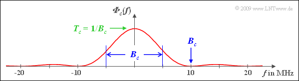
(2) By definition, with $T_c = T/100 = 0.1\ \rm µ s$:

Power density spectrum of the pseudo-noise spread signal
- $$B_c= \frac{1}{T_c} \cdot \hspace{-0.03cm} \int_{-\infty }^{+\infty} \hspace{-0.03cm} {\it \Phi}_{c}(f)\hspace{0.1cm} {\rm d}f = \hspace{-0.03cm} \int_{-\infty }^{+\infty} \hspace{-0.03cm} {\rm sinc}^2 \left(f T_c \right )\hspace{0.1cm} {\rm d}f $$
- $$\Rightarrow \hspace{0.3cm} B_c= \frac{1}{T_c}\hspace{0.15cm}\underline {= 10\,{\rm MHz}} \hspace{0.05cm}$$
The graph illustrates,
- that $B_c$ is given by the first zero of the $\rm sinc^2$ function in the equivalent low-pass range,
- but at the same time also gives the equivalent (equal area) bandwidth in the band-pass region.
(3) Solutions 2 and 5 are correct:
- The PDS ${\it \Phi}_s(f)$ results from the convolution of ${\it \Phi}_q(f)$ and ${\it \Phi}_c(f)$. This actually gives $B_s = B_c + B$ for the bandwidth of the transmitted signal.
- Since the spreading signal $c(t) ∈ \{+1, –1\}$ multiplied by itself always gives the value $1$, naturally $b(t) ≡ q(t)$ and consequently $B_b = B$.
- Obviously, the bandwidth $B_b$ of the band compressed signal is not equal to $2B_c + B$, although the convolution ${\it \Phi}_s(f) ∗ {\it \Phi}_c(f)$ suggests this.
- This is due to the fact that the power density spectra must not be convolved, but the spectral functions (amplitude spectra) $S(f)$ and $C(f)$ must be assumed, taking into account the phase relations.
- Only then can the PDS $B(f)$ be determined from ${\it \Phi}_b(f)$. Clearly, the following is also true: $C(f) ∗ C(f) = δ(f)$.
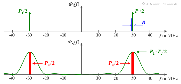
(4) Only the first solution is correct. The solution shall be clarified by the diagram at the end of the page:
- In the upper diagram the PDS ${\it \Phi}_i(f)$ of the narrowband interferer is approximated by two Dirac delta functions at $±f_{\rm T}$ with weights $P_{\rm I}/2$. Also plotted is the bandwidth $B = 0.1 \ \rm MHz$ (not quite true to scale).
- The receiver-side multiplication with $c(t)$ – actually with the function of the band compression, at least with respect to the useful part of $r(t)$ – causes a band spreading with respect to the interference signal $i(t)$. Without considering the useful signal, $b(t) = n(t) = i(t) · c(t)$. It follows:
- $${\it \Phi}_{n}(f) = {\it \Phi}_{i}(f) \star {\it \Phi}_{c}(f) = \frac{P_{\rm I}\cdot T_c}{2}\cdot {\rm sinc}^2 \left( (f - f_{\rm T}) \cdot T_c \right )+ \frac{P_{\rm I}\cdot T_c}{2}\cdot {\rm sinc}^2 \left( (f + f_{\rm T}) \cdot T_c \right ) \hspace{0.05cm}.$$

Power density spectra before and after band spreading
- Note that $n(t)$ is used here only as an abbreviation and does not denote AWGN noise.
- In a narrow range around the carrier frequency $f_{\rm T} = 30 \ \rm MHz$, the PDS ${\it \Phi}_n(f)$ is almost constant. Thus, the interference power after band spreading is:
- $$ P_{n} = P_{\rm I} \cdot T_c \cdot B = P_{\rm I}\cdot \frac{B}{B_c} = \frac{P_{\rm I}}{J}\hspace{0.05cm}. $$
- This means: The interference power is reduced by the factor $J = T/T_c$ by band spreading, which is why $J$ is often called "spreading gain".
- However, such a "spreading gain" is only given for a narrowband interferer.