Difference between revisions of "Digital Signal Transmission/Burst Error Channels"
| Line 578: | Line 578: | ||
{\big [ 1 -(1- {p_{\rm S} }^{1/\alpha})\big ]^{-2\alpha} } \hspace{0.05cm}.</math> | {\big [ 1 -(1- {p_{\rm S} }^{1/\alpha})\big ]^{-2\alpha} } \hspace{0.05cm}.</math> | ||
| − | * | + | *Thus, with the [[Digital_Signal_Transmission/Burst_Error_Channels#Error_distance_consideration_to_the_Wilhelm_model|"specific error distance distribution"]] $V_a(z)$, we obtain the following final result: |
::<math>p_1 = p_{\rm S} | ::<math>p_1 = p_{\rm S} | ||
| Line 585: | Line 585: | ||
(1- {p_{\rm S} }^{1/\alpha})^{n-1} \hspace{0.05cm}.</math>}}<br> | (1- {p_{\rm S} }^{1/\alpha})^{n-1} \hspace{0.05cm}.</math>}}<br> | ||
| − | [[File:P ID2836 Dig T 5 3 S5 Analyse2 neu.png|right|frame| | + | [[File:P ID2836 Dig T 5 3 S5 Analyse2 neu.png|right|frame|Mean number of errors in the burst of length $k$]] |
{{GraueBox|TEXT= | {{GraueBox|TEXT= | ||
| − | $\text{ | + | $\text{Example 11:}\ \text{Mean number of errors } {\rm E}[G_{\rm Burst}] \text{ in a burst with end parameter }k_{\rm Burst}$ |
| − | + | Let the mean symbol error probability still be $p_{\rm S} = 10^{-3}$, i.e. (relatively) small.<br> | |
| − | '''(1) | + | '''(1) Red curve for the BSC channel (or $\alpha = 1)$''': |
| − | * | + | * For example, the parameter $k_{\rm Burst}= 10$ means that the burst is finished when nine error-free symbols follow after one error. The probability for an error distance $a \le 9$ is extremely small when $p_{\rm S}$ is small $($hier: $10^{-3})$ äußerst klein. Daraus folgt weiter, dass dann (fast) jeder Einzelfehler als ein "Burst" aufgefasst wird, und es gilt ${\rm E}[G_{\rm Burst}] \approx 1.01$ .<br> |
* Bei größerem Burst–Endeparameter $k_{\rm Burst}$ nimmt auch die Wahrscheinlichkeit ${\rm Pr}(a \le k_{\rm Burst})$ deutlich zu und es kommt zu "Bursts" mit mehr als einem Fehler. Wählt man beispielsweise $k_{\rm Burst}= 100$, so beinhaltet ein "Burst" im Mittel $1.1$ Symbolfehler.<br> | * Bei größerem Burst–Endeparameter $k_{\rm Burst}$ nimmt auch die Wahrscheinlichkeit ${\rm Pr}(a \le k_{\rm Burst})$ deutlich zu und es kommt zu "Bursts" mit mehr als einem Fehler. Wählt man beispielsweise $k_{\rm Burst}= 100$, so beinhaltet ein "Burst" im Mittel $1.1$ Symbolfehler.<br> | ||
*Das bedeutet gleichzeitig, dass es auch beim BSC–Modell zu langen Fehlerbursts (entsprechend unserer Definition) kommen kann, wenn bei gegebenem $p_{\rm S}$ der Burst–Endeparameter zu groß gewählt ist oder bei vorgegebenem $k_{\rm Burst}$ die mittlere Fehlerwahrscheinlichkeit $p_{\rm S}$ zu groß ist.<br><br> | *Das bedeutet gleichzeitig, dass es auch beim BSC–Modell zu langen Fehlerbursts (entsprechend unserer Definition) kommen kann, wenn bei gegebenem $p_{\rm S}$ der Burst–Endeparameter zu groß gewählt ist oder bei vorgegebenem $k_{\rm Burst}$ die mittlere Fehlerwahrscheinlichkeit $p_{\rm S}$ zu groß ist.<br><br> | ||
Revision as of 13:48, 2 September 2022
Contents
- 1 Channel model according to Gilbert-Elliott
- 2 Error distance distribution of the GE model
- 3 Error correlation function of the GE model
- 4 Channel model according to McCullough
- 5 Conversion of the GE parameters into the MC parameters
- 6 Burst error channel model according to Wilhelm
- 7 Error distance consideration to the Wilhelm model
- 8 Numerical comparison of the BSC model and the Wilhelm model
- 9 Error distance consideration according to the Wilhelm A model
- 10 Error correlation function of the Wilhelm A model
- 11 Analysis of error structures with the Wilhelm A model
- 12 Aufgaben zum Kapitel
- 13 Quellenverzeichnis
Channel model according to Gilbert-Elliott
This channel model, which goes back to "E. N. Gilbert" [Gil60][1] and E. O. Elliott [Ell63][2], is suitable for describing and simulating digital transmission systems with burst error characteristics.
The Gilbert–Elliott model (abbreviation: GE model) can be characterized as follows:
- The different transmission quality at different times is expressed by a finite number $g$ of channel states $(Z_1, Z_2,\hspace{0.05cm} \text{...} \hspace{0.05cm}, Z_g)$.
- The in reality smooth transitions of the noise intensity – in the extreme case from completely error-free transmission to total failure – are approximated in the GE model by fixed probabilities in the individual channel states.
- The transitions between the $g$ states occur according to a "Markov process" (1st order) and are characterized by $g \cdot (g-1)$ transition probabilities. Together with the $g$ error probabilities in the individual states, there are thus $g^2$ free model parameters.
- For reasons of mathematical manageability, one usually restricts oneself to $g = 2$ states and denotes these with $\rm G$ ("GOOD") and $\rm B$ ("BAD"). Mostly, the error probability in state $\rm G$ will be much smaller than in state $\rm B$.
- In what follows, we use these two error probabilities $p_{\rm G}$ and $p_{\rm B}$, where $p_{\rm G} < p_{\rm B}$ should hold, as well as the transition probabilities ${\rm Pr}({\rm B}\hspace{0.05cm}|\hspace{0.05cm}{\rm G})$ and ${\rm Pr}({\rm G}\hspace{0.05cm}|\hspace{0.05cm}{\rm B})$. This also determines the other two transition probabilities:
- \[{\rm Pr}(\rm G\hspace{0.05cm}|\hspace{0.05cm} G) = 1 - {\rm Pr}(\rm B\hspace{0.05cm}|\hspace{0.05cm} G), \hspace{0.2cm} {\rm Pr}(\rm B\hspace{0.05cm}|\hspace{0.05cm} B) = 1 - {\rm Pr}(\rm G\hspace{0.05cm}|\hspace{0.05cm} B)\hspace{0.05cm}.\]
$\text{Example 1:}$ We consider the GE model with the parameters
- $$p_{\rm G} = 0.01,$$
- $$p_{\rm B} = 0.4,$$
- $${\rm Pr}(\rm G\hspace{0.05cm}\vert\hspace{0.05cm} B) = 0.1, $$
- $$ {\rm Pr}(\rm B\hspace{0.05cm}\vert\hspace{0.05cm} G) = 0.01\hspace{0.05cm}.$$
The underlying model is shown at the end of the example with the parameters given here.
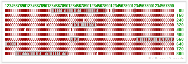
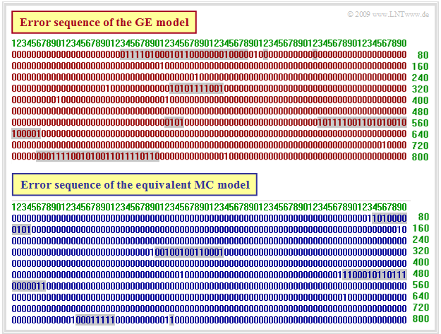
The upper graphic shows a (possible) error sequence of length $N = 800$. If the GE model is in the "BAD" state, this is indicated by the gray background.
To simulate such a GE error sequence, switching is performed between the states "GOOD" and "BAD" according to the four transition probabilities.
- At the first clock call, the selection of the state is expediently done according to the probabilities $w_{\rm G}$ and $w_{\rm B}$, as calculated below.
- At each clock cycle exactly one element of the error sequence $ \langle e_\nu \rangle$ is generated according to the current error probability $(p_{\rm G}$ or $p_{\rm B})$.
- The "error distance simulation" is not applicable here, because in the GE model a state change is possible after each symbol (and not only after an error).
The probabilities that the Markov chain is in the "GOOD" or "BAD" state can be calculated from the assumed homogeneity and stationarity. One obtains with the above numerical values:
- \[w_{\rm G} = {\rm Pr(in\hspace{0.15cm} state \hspace{0.15cm}G)}= \frac{ {\rm Pr}(\rm G\hspace{0.05cm}\vert\hspace{0.05cm} B)}{ {\rm Pr}(\rm G\hspace{0.05cm}\vert\hspace{0.05cm} B) + {\rm Pr}(\rm B\hspace{0.05cm}\vert\hspace{0.05cm} G)} = \frac{0.1}{0.1 + 0.01} = {10}/{11}\hspace{0.05cm},\]
- \[w_{\rm B} = {\rm Pr(in\hspace{0.15cm} state \hspace{0.15cm}B)}= \frac{ {\rm Pr}(\rm B\hspace{0.05cm}\vert\hspace{0.05cm} G)}{ {\rm Pr}(\rm G\hspace{0.05cm}\vert\hspace{0.05cm} B) + {\rm Pr}(\rm B\hspace{0.05cm}\vert\hspace{0.05cm} G)} = \frac{0.11}{0.1 + 0.01} = {1}/{11}\hspace{0.05cm}.\]
These two state probabilities can also be used to determine the average error probability of the GE model:
- \[p_{\rm M} = w_{\rm G} \cdot p_{\rm G} + w_{\rm B} \cdot p_{\rm B} = \frac{p_{\rm G} \cdot {\rm Pr}({\rm G\hspace{0.05cm}\vert\hspace{0.05cm} B)}+ p_{\rm B} \cdot {\rm Pr}(\rm B\hspace{0.05cm}\vert\hspace{0.05cm} G)}{ {\rm Pr}(\rm G\hspace{0.05cm}\vert\hspace{0.05cm} B) + {\rm Pr}(\rm B\hspace{0.05cm}\vert\hspace{0.05cm} G)} \hspace{0.05cm}.\]
In particular, for the model considered here as an example:
- \[p_{\rm M} ={10}/{11} \cdot 0.01 +{1}/{11} \cdot 0.4 = {1}/{22} \approx 4.55\%\hspace{0.05cm}.\]
Error distance distribution of the GE model
In [Hub82][3] you can find the analytical computations
- of the probability of the error distance $k$:
- \[{\rm Pr}(a=k) = \alpha_{\rm G} \cdot \beta_{\rm G}^{\hspace{0.05cm}k-1} \cdot (1- \beta_{\rm G}) + \alpha_{\rm B} \cdot \beta_{\rm B}^{\hspace{0.05cm}k-1} \cdot (1- \beta_{\rm B})\hspace{0.05cm},\]
- \[V_a(k) = {\rm Pr}(a \ge k) = \alpha_{\rm G} \cdot \beta_{\rm G}^{\hspace{0.05cm}k-1} + \alpha_{\rm B} \cdot \beta_{\rm B}^{\hspace{0.05cm}k-1} \hspace{0.05cm}.\]
The following auxiliary quantities are used here:
- \[u_{\rm GG} ={\rm Pr}(\rm G\hspace{0.05cm}|\hspace{0.05cm} G ) \cdot (1-{\it p}_{\rm G}) \hspace{0.05cm},\hspace{0.2cm} {\it u}_{\rm GB} ={\rm Pr}(\rm B\hspace{0.05cm}|\hspace{0.05cm} G ) \cdot (1-{\it p}_{\hspace{0.03cm} \rm G}) \hspace{0.05cm},\]
- \[u_{\rm BB} ={\rm Pr}(\rm B\hspace{0.05cm}|\hspace{0.05cm} B ) \cdot (1-{\it p}_{\hspace{0.03cm}\rm B}) \hspace{0.05cm},\hspace{0.29cm} {\it u}_{\rm BG} ={\rm Pr}(\rm G\hspace{0.05cm}|\hspace{0.05cm} B ) \cdot (1-{\it p}_{\hspace{0.03cm}\rm B})\hspace{0.05cm}\]
- \[\Rightarrow \hspace{0.3cm} \beta_{\rm G} =\frac{u_{\rm GG} + u_{\rm BB} + \sqrt{(u_{\rm GG} - u_{\rm BB})^2 + 4 \cdot u_{\rm GB}\cdot u_{\rm BG}}}{2} \hspace{0.05cm},\]
- \[\hspace{0.8cm}\beta_{\rm B} =\frac{u_{\rm GG} + u_{\rm BB} - \sqrt{(u_{\rm GG} - u_{\rm BB})^2 + 4 \cdot u_{\rm GB}\cdot u_{\rm BG}}}{2}\hspace{0.05cm}.\]
- \[x_{\rm G} =\frac{u_{\rm BG}}{\beta_{\rm G}-u_{\rm BB}} \hspace{0.05cm},\hspace{0.2cm} x_{\rm B} =\frac{u_{\rm BG}}{\beta_{\rm B}-u_{\rm BB}}\]
- \[\Rightarrow \hspace{0.3cm} \alpha_{\rm G} = \frac{(w_{\rm G} \cdot p_{\rm G} + w_{\rm B} \cdot p_{\rm B}\cdot x_{\rm G})( x_{\rm B}-1)}{p_{\rm M} \cdot( x_{\rm B}-x_{\rm G})} \hspace{0.05cm}, \hspace{0.2cm}\alpha_{\rm B} = 1-\alpha_{\rm G}\hspace{0.05cm}.\]
The given equations are the result of extensive matrix operations.
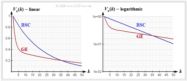
The upper graph shows the error distance distribution (EDD) of the GE model (red curve) in linear and logarithmic representation for the parameters
- $${\rm Pr}(\rm G\hspace{0.05cm}|\hspace{0.05cm} B ) = 0.1 \hspace{0.05cm},\hspace{0.5cm}{\rm Pr}(\rm B\hspace{0.05cm}|\hspace{0.05cm} G ) = 0.001 \hspace{0.05cm},\hspace{0.5cm}p_{\rm B} = 0.4.$$
For comparison, the corresponding $V_a(k)$ curve for the BSC model with the same mean error probability $p_{\rm M} = 4.5\%$ is also plotted as a blue curve.
Error correlation function of the GE model
For the "error correlation function" (ECF) of the GE model with
- the mean error probability $p_{\rm M}$,
- the transition probabilities ${\rm Pr}(\rm B\hspace{0.05cm}|\hspace{0.05cm} G )$ and ${\rm Pr}(\rm G\hspace{0.05cm}|\hspace{0.05cm} B )$ as well as
- the error probabilities $p_{\rm G}$ and $p_{\rm B}$ in the two states $\rm G$ and $\rm B$
we obtain after extensive matrix operations the relatively simple expression
- \[\varphi_{e}(k) = {\rm E}\big[e_\nu \cdot e_{\nu +k}\big] = \left\{ \begin{array}{c} p_{\rm M} \\ p_{\rm M}^2 + (p_{\rm B} - p_{\rm M}) (p_{\rm M} - p_{\rm G}) [1 - {\rm Pr}(\rm B\hspace{0.05cm}|\hspace{0.05cm} G )- {\rm Pr}(\rm G\hspace{0.05cm}|\hspace{0.05cm} B )]^k \end{array} \right.\quad \begin{array}{*{1}c} f{\rm or }\hspace{0.15cm}k = 0 \hspace{0.05cm}, \\ f{\rm or }\hspace{0.15cm} k > 0 \hspace{0.05cm}.\\ \end{array}\]
For the GE model, $\varphi_{e}(k)$ must always be calculated according to this equation. The iterative calculation algorithm
- $$\varphi_{e}(k) = \sum_{\kappa = 1}^{k} {\rm Pr}(a = \kappa) \cdot \varphi_{e}(k - \kappa) $$
which is only valid for "renewing models", cannot be applied here, since the GE model is not renewing ⇒ The error distances are not statistically independent of each other here.
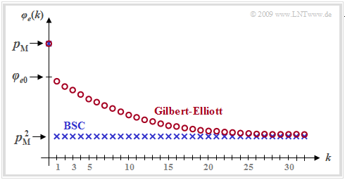
The graph shows an example of the ECF curve of the GE model marked with red circles. One can see from this representation:
- While for the memoryless channel (BSC model, blue curve) all ECF values are $\varphi_{e}(k \ne 0)= p_{\rm M}^2$ for the burst error channel the ECF values approach this final value much more slowly.
- At the transition from $k = 0$ to $k = 1$ a certain discontinuity occurs. While $\varphi_{e}(k = 0)= p_{\rm M}$, the second equation valid for $k > 0$ yields the following extrapolated value for $k = 0$:
- \[\varphi_{e0} = p_{\rm M}^2 + (p_{\rm B} - p_{\rm M}) \cdot (p_{\rm M} - p_{\rm G})\hspace{0.05cm}.\]
- A quantitative measure of the length of the statistical ties is the correlation duration $D_{\rm K}$, which is generally defined as the width of an equal-area rectangle of height $\varphi_{e0} - p_{\rm M}^2$:
- \[D_{\rm K} = \frac{1}{\varphi_{e0} - p_{\rm M}^2} \cdot \sum_{k = 1 }^{\infty}\hspace{0.1cm} \big[\varphi_{e}(k) - p_{\rm M}^2\big ]\hspace{0.05cm}.\]
$\text{Conclusion:}$ In the Gilbert–Elliott model, the correlation term is given by the simple, analytically expressible expression
- \[D_{\rm K} =\frac{1}{ {\rm Pr}(\rm G\hspace{0.05cm}\vert\hspace{0.05cm} B ) + {\rm Pr}(\rm B\hspace{0.05cm}\vert\hspace{0.05cm} G )}-1 \hspace{0.05cm}.\]
- $D_{\rm K}$ is larger the smaller ${\rm Pr}(\rm B\hspace{0.05cm}\vert\hspace{0.05cm} G )$ and ${\rm Pr}(\rm G\hspace{0.05cm}\vert\hspace{0.05cm}B )$ are, i.e., when state changes occur rarely.
- For the BSC model ⇒ $p_{\rm B}= p_{\rm G} = p_{\rm M}$ ⇒ $D_{\rm K} = 0$ this equation is not applicable.
Channel model according to McCullough
The main disadvantage of the GE model is that it does not allow error distance simulation. As will be worked out in "Exercise 5.5", this has great advantages over the symbol-wise generation of the error sequence $\langle e_\nu \rangle$ in terms of computational speed and memory requirements.
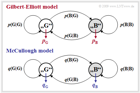
McCullough [McC68][4] modified the model developed three years earlier by Gilbert and Elliott so that an error distance simulation in the two states "GOOD" and "BAD" is applicable in each case by itself. The graph below shows McCullough's model, hereafter referred to as the MC model, while the GE model is shown above after renaming the transition probabilities ⇒ ${\rm Pr}(\rm B\hspace{0.05cm}\vert\hspace{0.05cm}G ) \rightarrow {\it p}(\rm G\hspace{0.05cm}\vert\hspace{0.05cm}B )$, ${\rm Pr}(\rm B\hspace{0.05cm}\vert\hspace{0.05cm}G ) \rightarrow {\it p}(\rm G\hspace{0.05cm}\vert\hspace{0.05cm}B )$, etc.
There are many similarities and a few differences between the two models:
- Like the Gilbert–Elliott model, the McCullough channel model is based on a first-order Markov process with the two states "GOOD" $(\rm G)$ and "BAD" $(\rm B)$. No difference can be found with respect to the model structure.
- The main difference to the GE model is that a change of state between "GOOD" and "BAD" is only possible after an error – i.e. a "$1$" in the error sequence. This enables a error distance simulation.
- The four freely selectable GE parameters $p_{\rm G}$, $p_{\rm B}$, ${\it p}(\rm B\hspace{0.05cm}\vert\hspace{0.05cm}G )$ and ${\it p}(\rm G\hspace{0.05cm}\vert\hspace{0.05cm}B )$ can – as shown on the next section – be converted into the MC parameters $q_{\rm G}$, $q_{\rm B}$, ${\it q}(\rm B\hspace{0.05cm}\vert\hspace{0.05cm}G )$ and ${\it q}(\rm G\hspace{0.05cm}\vert\hspace{0.05cm}B )$ in such a way that a error sequence with the same statistical properties as in the GE model is generated.
- For example, ${\it q}(\rm B\hspace{0.05cm}\vert\hspace{0.05cm}G )$ denotes the transition probability from the "GOOD" state to the "BAD" state under the condition that an error has just occurred in the "GOOD" state. The GE parameter ${\it p}(\rm B\hspace{0.05cm}\vert\hspace{0.05cm}G )$ characterizes this transition probability without this additional condition.
$\text{Example 2:}$ The figure above shows an exemplary error sequence of the GE model with the parameters $p_{\rm G} = 0.01$, $p_{\rm B} = 0.4$, ${\it p}(\rm B\hspace{0.05cm}\vert\hspace{0.05cm}G ) = 0.01$, ${\it p}(\rm G\hspace{0.05cm}\vert\hspace{0.05cm}B ) = 0.1$. It can be seen that, in contrast to the lower MC sequence, a change of state from "GOOD" (without background) to "BAD" (gray background) and vice versa is possible at any time $\nu$ – i.e. even when $e_\nu = 0$.
$\text{Conclusion:}$ The correlations between the two models can be summarized as follows:
- In the error sequence of the McCullough model shown in the example below, in contrast to the upper sequence, a change of state at time $\nu$ is only possible at $e_\nu = 1$. The last error value before a gray background is always a "$1$".
- This has the advantage that one does not have to generate the errors "step–by–step" in an error sequence simulation, but can use the faster error distance simulation ⇒ see "Exercise 5.5".
- The parameters of the GE model can be converted into corresponding MC parameters in such a way that the two models are equivalent ⇒ see next section. That means: The MC error sequence has exactly the same statistical properties as the GE error sequence. However, it does not mean that both error sequences are identical.
Conversion of the GE parameters into the MC parameters
The parameters of the equivalent MC model can be calculated from the GE parameters as follows:
- \[q_{\rm G} =1-\beta_{\rm G}\hspace{0.05cm}, \hspace{0.9cm}q_{\rm B} = 1-\beta_{\rm B}\hspace{0.05cm}, \hspace{0.9cm}q(\rm B\hspace{0.05cm}|\hspace{0.05cm} G ) =\frac{\alpha_{\rm B} \cdot[{\rm Pr}(\rm B\hspace{0.05cm}|\hspace{0.05cm} G ) + {\rm Pr}(\rm G\hspace{0.05cm}|\hspace{0.05cm} B )]}{\alpha_{\rm G} \cdot q_{\rm B} + \alpha_{\rm B} \cdot q_{\rm G}} \hspace{0.05cm}, \hspace{0.9cm} q(\rm G\hspace{0.05cm}|\hspace{0.05cm} B ) = \frac{\alpha_{\rm G}}{\alpha_{\rm B}} \cdot q(\rm B\hspace{0.05cm}|\hspace{0.05cm} G )\hspace{0.05cm}.\]
Here again the following auxiliary quantities are used:
- \[u_{\rm GG} = {\rm Pr}(\rm G\hspace{0.05cm}|\hspace{0.05cm} G ) \cdot (1-{\it p}_{\rm G}) \hspace{0.05cm},\hspace{0.2cm} {\it u}_{\rm GB} ={\rm Pr}(\rm B\hspace{0.05cm}|\hspace{0.05cm} G ) \cdot (1-{\it p}_{\hspace{0.03cm} \rm G}) \hspace{0.05cm},\]
- \[u_{\rm BB} = {\rm Pr}(\rm B\hspace{0.05cm}|\hspace{0.05cm} B ) \cdot (1-{\it p}_{\hspace{0.03cm}\rm B}) \hspace{0.05cm},\hspace{0.29cm} {\it u}_{\rm BG} ={\rm Pr}(\rm G\hspace{0.05cm}|\hspace{0.05cm} B ) \cdot (1-{\it p}_{\hspace{0.03cm}\rm B})\]
- \[\Rightarrow \hspace{0.3cm} \beta_{\rm G} = \frac{u_{\rm GG} + u_{\rm BB} + \sqrt{(u_{\rm GG} - u_{\rm BB})^2 + 4 \cdot u_{\rm GB}\cdot u_{\rm BG}}}{2} \hspace{0.05cm}, \hspace{0.9cm}\beta_{\rm B} \hspace{-0.1cm} = \hspace{-0.1cm}\frac{u_{\rm GG} + u_{\rm BB} - \sqrt{(u_{\rm GG} - u_{\rm BB})^2 + 4 \cdot u_{\rm GB}\cdot u_{\rm BG}}}{2}\hspace{0.05cm}.\]
- \[x_{\rm G} =\frac{u_{\rm BG}}{\beta_{\rm G}-u_{\rm BB}} \hspace{0.05cm},\hspace{0.2cm} x_{\rm B} =\frac{u_{\rm BG}}{\beta_{\rm B}-u_{\rm BB}} \Rightarrow \hspace{0.3cm} \alpha_{\rm G} = \frac{(w_{\rm G} \cdot p_{\rm G} + w_{\rm B} \cdot p_{\rm B}\cdot x_{\rm G})( x_{\rm B}-1)}{p_{\rm M} \cdot( x_{\rm B}-x_{\rm G})} \hspace{0.05cm}, \hspace{0.9cm}\alpha_{\rm B} = 1-\alpha_{\rm G}\hspace{0.05cm}.\]
$\text{Example 3:}$ As in $\text{Example 2}$, the GE parameters are:
- $$p_{\rm G} = 0.01, \hspace{0.5cm} p_{\rm B} = 0.4, \hspace{0.5cm} p(\rm B\hspace{0.05cm}\vert\hspace{0.05cm}G ) = 0.01, \hspace{0.5cm} {\it p}(\rm G\hspace{0.05cm}\vert\hspace{0.05cm}B ) = 0.1.$$
Applying the above equations, we then obtain for the equivalent MC parameters:
- $$q_{\rm G} = 0.0186, \hspace{0.5cm} q_{\rm B} = 0.4613, \hspace{0.5cm} q(\rm B\hspace{0.05cm}\vert\hspace{0.05cm}G ) = 0.3602, \hspace{0.5cm} {\it q}(\rm G\hspace{0.05cm}\vert\hspace{0.05cm}B ) = 0.2240.$$
- If we compare in $\text{Example 2}$ the red error sequence (GE, change of state is always possible) with the blue sequence (equivalent MC, change of state only at $e_\nu = 1$), we can see quite serious differences.
- But the blue error sequence of the equivalent McCullough model has exactly the same statistical properties as the red error sequence of the Gilbert-Elliott model.
The conversion of the GE parameters to the MC parameters is illustrated in "Exercise 5.7" using a simple example. "Exercise 5.7Z" further shows how the mean error probability, the error distance distribution, the error correlation function and the correlation duration of the MC model can be determined directly from the $q$ parameters.
Burst error channel model according to Wilhelm
This model goes back to "Claus Wilhelm" and was developed from the mid-1960s onwards from empirical measurements of temporal consequences of bit errors. It is based on thousands of measurement hours in transmission channels from $\text{200 bit/s}$ with analog modem up to $\text{2.048 Mbit/s}$ via "ISDN". Likewise, marine radio channels up to $7500$ kilometers in the shortwave range were measured.
Blocks of length $n$ were recorded. The respective block error rate $h_{\rm B}(n)$ was determined from this.
- A block error is already present if even one of the $n$ symbols has been falsified.
- Knowing well that the block error rate $h_{\rm B}(n)$ corresponds exactly to the block error probability $p_{\rm B}$ only for $n \to \infty$, we set $p_{\rm B}(n) \approx h_{\rm B}(n)$ in the following description.
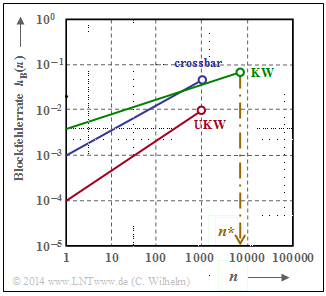
In a large number of measurements, the fact that the course $p_{\rm B}(n)$ in double-logarithmic representation show linear increases in the lower range has been confirmed again and again (see graph). Thus, it holds for $n \le n^\star$:
- \[{\rm lg} \hspace{0.15cm}p_{\rm B}(n) = {\rm lg} \hspace{0.15cm}p_{\rm S} + \alpha \cdot {\rm lg} \hspace{0.15cm}n\hspace{0.3cm} \Rightarrow \hspace{0.3cm} p_{\rm B}(n) = p_{\rm S} \cdot n^{\alpha}\hspace{0.05cm}.\]
Here, $p_{\rm S} = p_{\rm B}(n=1)$ denotes the mean symbol error probability and the empirically found values of $\alpha$ are between $0.5$ and $0.95$. For $1-\alpha$, the term burst factor is also used.
Note that $p_{\rm B}(n)$ indicates the block error probability. In another context, $p_{\rm B}$ sometimes also denotes the bit error probability in our learning tutorial.
$\text{Example 4:}$ In the BSC model, the course of the block error probability is:
- \[p_{\rm B}(n) =1 -(1 -p_{\rm S})^n \approx n \cdot p_{\rm S}\hspace{0.05cm}.\]
From this follows $\alpha = 1$ resp. the burst factor $1-\alpha = 0$. In this case (and only in this case) a linear course results even with non-logarithmic representation.
- Note that the above approximation is only valid for $p_{\rm S} \ll 1$ and not too large $n$, otherwise the approximation $(1-p_{\rm S})^n \approx1 - n \cdot p_{\rm S}$ is not applicable.
- But this also means that the equation given above is also only valid for a lower range $($for $n < n^\star)$.
- Otherwise, an infinitely large block error probability would result for $n \to \infty$.
$\text{Definition:}$ For the function $p_{\rm B}(n)$ determined empirically from measurements, we now have to find the error distance distribution from which the course for $n > n^\star$ can be extrapolated, which satisfies the following constraint:
- \[\lim_{n \hspace{0.05cm} \rightarrow \hspace{0.05cm} \infty} p_{\rm B}(n) = 1 .\]
We refer to this approach as the Wilhelm model. Since memory extends only to the last symbol error, this model is renewal model..
Error distance consideration to the Wilhelm model
We now consider the error distances. An error sequence $\langle e_\nu \rangle$ can be equivalently represented by the error distance sequence $\langle a_{\nu\hspace{0.06cm}'} \rangle$, as shown in the following graph. It can be seen:
- The error sequence $\text{...}\rm 1001\text{...}$ is expressed by $a= 3$.
- Accordingly, the error distance $a= 1$ denotes the error sequence $\text{...}\rm 11\text{...}$.
- The different indices $\nu$ and $\nu\hspace{0.06cm}'$ take into account that the two sequences do not run synchronously.
With the probabilities $p_a(k) = {\rm Pr}(a= k)$ for the individual error distances $k$ and the mean (symbol) error probability $p_{\rm S}$, the following definitions apply for
- the error distance distribution (EDD):
- \[ V_a(k) = {\rm Pr}(a \ge k)= \sum_{\kappa = k}^{\infty}p_a(\kappa) \hspace{0.05cm},\]
- the mean error distance ${\rm E}\big[a\big]$:
- \[ V_a(k) = {\rm E}\big[a\big] = \sum_{k = 1}^{\infty} k \cdot p_a(k) = {1}/{p_{\rm S}}\hspace{0.05cm}.\]
$\text{Example 5:}$ We consider a block with $n$ bits, starting at bit position $\nu + 1$.
- A block error occurs whenever a bit is falsified at positions $\nu + 1$, ... , $\nu + n$.
- The falsification probabilities are expressed in the graph by the error distance distribution ${V_a}\hspace{0.06cm}'(k)$.
- Somewhere before the block of length $n = 3$ is the last error, but at least at distance $k$ from the first error in the block.
- So the distance is equal or greater than $k$, which corresponds exactly to the probability ${V_a}'(k)$.
- The apostrophe is to indicate that a correction has to be made later to get from the empirically found EDD to the correct function ${V_a}(k)$.
We now have several equations for the block error probability $p_{\rm B}(n)$.
- A first equation establishes the relationship between $p_{\rm B}(n)$ and the (approximate) error distance distribution ${V_a}'(k)$:
- \[(1)\hspace{0.4cm} p_{\rm B}(n) = p_{\rm S} \cdot \sum_{k = 1}^{n} V_a\hspace{0.05cm}'(k) \hspace{0.05cm}, \]
- A second equation is provided by our empirical investigation at the beginning of this section:
- \[(2)\hspace{0.4cm} p_{\rm B}(n) = p_{\rm S} \cdot n^{\alpha}\]
- The third equation is obtained by equating $(1)$ and $(2)$:
- \[(3)\hspace{0.4cm} \sum_{k = 1}^{n} V_a\hspace{0.05cm}'(k) = n^{\alpha} \hspace{0.05cm}. \]
By successively substituting $n = 1, 2, 3,$ ... into this equation, we obtain with ${V_a}'(k = 1) = 1$:
- \[V_a\hspace{0.05cm}'(1) = 1^{\alpha} \hspace{0.05cm},\hspace{0.8cm} V_a\hspace{0.05cm}'(1) + V_a\hspace{0.05cm}'(2) =2^{\alpha} \hspace{0.05cm}, \hspace{0.8cm}V_a\hspace{0.05cm}'(1) + V_a\hspace{0.05cm}'(2) + V_a\hspace{0.05cm}'(3) = 3^{\alpha} \hspace{0.35cm}\Rightarrow \hspace{0.3cm} V_a\hspace{0.05cm}'(k) = k^{\alpha}-(k-1)^{\alpha} \hspace{0.05cm}.\]
However, the coefficients ${V_a}'(k)$ obtained from empirical data do not necessarily satisfy the normalization condition.
To correct the issue, Wilhelm uses the following approach:
- \[V_a\hspace{0.05cm}(k) = V_a\hspace{0.05cm}'(k) \cdot {\rm e}^{- \beta \cdot (k-1)}\hspace{0.3cm}\Rightarrow \hspace{0.3cm} V_a\hspace{0.05cm}(k) = \big [k^{\alpha}-(k-1)^{\alpha} \big ] \cdot {\rm e}^{- \beta \cdot (k-1)}\hspace{0.05cm}.\]
Wilhelm refers to this representation as the L–model, see [Wil11][5]. The constant $\beta$ is dependent on
- the symbol error probability $p_{\rm S}$, and
- the empirically found exponent $\alpha$ ⇒ burst factor $1- \alpha$
such that the block error probability becomes equal to $1$ at infinite block length:
- \[\lim_{n \hspace{0.05cm} \rightarrow \hspace{0.05cm} \infty} p_B(n) = p_{\rm S} \cdot \sum_{k = 1}^{n} V_a\hspace{0.05cm}(k) = p_{\rm S} \cdot \sum_{k = 1}^{n} \big [k^{\alpha}-(k-1)^{\alpha} \big ] \cdot {\rm e}^{- \beta \cdot (k-1)} =1 \hspace{0.3cm} \Rightarrow \hspace{0.3cm} \sum_{k = 1}^{\infty} \big [k^{\alpha}-(k-1)^{\alpha} \big ] \cdot {\rm e}^{- \beta \cdot (k-1)} = {1}/{p_{\rm S}} \hspace{0.05cm}.\]
To determine $\beta$, we use the "generating function" of ${V_a}(k)$, which we denote by ${V_a}(z)$:
- \[V_a\hspace{0.05cm}(z) = \sum_{k = 1}^{\infty}V_a\hspace{0.05cm}(k) \cdot z^k = \sum_{k = 1}^{n} \big [k^{\alpha}-(k-1)^{\alpha} \big ] \cdot {\rm e}^{- \beta \cdot (k-1)} \cdot z^k \hspace{0.05cm}.\]
In [Wil11][5], $V_a\hspace{0.05cm}(z) = 1/{\left (1- {\rm e}^{- \beta }\cdot z \right )^\alpha} $ is derived approximately. From the equation for the mean error distance follows:
- \[ {\rm E}\big[a\big] = \sum_{k = 1}^{\infty} k \cdot p_a(k) = \sum_{k = 1}^{\infty} V_a(k) = \sum_{k = 1}^{\infty} V_a(k) \cdot 1^k = V_a(z=1) = 1/p_{\rm S}\]
- \[ \Rightarrow \hspace{0.3cm}{p_{\rm S}} = \big [V_a(z=1)\big]^{-1}= \big [1- {\rm e}^{- \beta }\cdot 1\big]^{\alpha}\hspace{0.3cm} \Rightarrow \hspace{0.3cm} {\rm e}^{- \beta } =1 - {p_{\rm S}}^{1/\alpha}\hspace{0.05cm}.\]
Numerical comparison of the BSC model and the Wilhelm model
$\text{Conclusion:}$ Let us summarize this intermediate result. Wilhelm's L–model describes the error distance distribution in the form
- \[V_a\hspace{0.05cm}(k) = \big [k^{\alpha}-(k-1)^{\alpha}\big ] \cdot \big [ 1 - {p_{\rm S}^{1/\alpha} }\big ]^{k-1} \hspace{0.05cm}.\]
This model will now be explained with exemplary numerical results.
$\text{Example 6:}$ We start with the "BSC model".
- For presentation reasons, we set the falsification probability very high to $p_{\rm S} = 0.2$.
- In the second row of the following table, its error distance distribution ${V_a}(k) = {\rm Pr}(a \ge k)$ is entered for $k \le10$.
The Wilhelm model with $p_{\rm S} = 0.2$ and $\alpha = 1$ has exactly the same error distance distribution ${V_a}(k)$ as the corresponding "BSC model". This is also shown by the calculation. With $\alpha = 1$ one obtains from the equation in the last section:
- \[V_a\hspace{0.05cm}(k) = \big [k^{\alpha}-(k-1)^{\alpha}\big ] \cdot \big [ 1 - {p_{\rm S}^{1/\alpha} }\big ]^{k-1} = (1 - p_{\rm S} )^{k-1} \hspace{0.05cm}.\]
Thus, according to lines 3 and 4, both models also have
- equal probabilities ${\rm Pr}(a = k)= {V_a}(k-1) - {V_a}(k)$ of the error distances,
- equal block error probabilities $ p_{\rm B}(n)$.
With regard to the following $\text{Example 7}$ with $\alpha \ne 1$, it should be mentioned again in particular:
- The block error probabilities $ p_{\rm B}(n)$ of the Wilhelm model are basically obtained from the error distance distribution ${V_a}(k)$ according to the equation
- \[ p_{\rm B}(n) = p_{\rm S} \cdot \sum_{k = 1}^{n} V_a\hspace{0.05cm}(k) \hspace{0.15cm}\Rightarrow \hspace{0.15cm} p_{\rm B}( 1) = 0.2 \cdot 1 = 0.2 \hspace{0.05cm}, \hspace{0.5cm}p_{\rm B}(2) = 0.2 \cdot (1+0.8) = 0.36 \hspace{0.05cm}.\]
- Only in the special case $\alpha = 1$ ⇒ BSC model, $ p_{\rm B}(n)$ can also be determined by summation over the error distance probabilities ${\rm Pr}(a=k)$:
- \[ p_{\rm B}(n) = p_{\rm S} \cdot \sum_{k = 1}^{n} {\rm Pr}(a=k) \hspace{0.15cm}\Rightarrow \hspace{0.15cm} p_{\rm B}( 1) = 0.2 \hspace{0.05cm}, \hspace{0.5cm}p_{\rm B}(2) = 0.2+ 0.16 = 0.36 \hspace{0.05cm}.\]
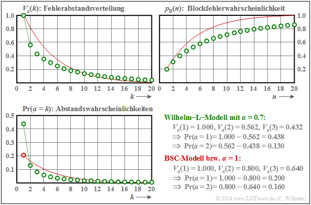
$\text{Example 7:}$ We now consider a channel with burst error characteristics.
- The graph shows as green circles the results for the Wilhelm–L model with $\alpha = 0.7$.
- The red comparison curve is valid for $\alpha = 1$ (or for the BSC channel) with the same mean symbol error probability $p_{\rm S} = 0.2$.
- Some interesting numerical values are given at the bottom right.
One can see from these plots:
- The course of the block error probability starts with $p_{\rm B}(n = 1) = p_{\rm S} = 0.2$, both for statistically independent errors (BSC) and for burst errors (Wilhelm).
- For the burst error channel, ${\rm Pr}(a=1)= 0.438$ is significantly larger than for the comparable BSC ⇒ ${\rm Pr}(a=1)= 0.2$. In addition, one can see a bent shape in the lower region.
- However, the mean error distance ${\rm E}\big [a \big ] = 1/p_{\rm S} = 5$ is also identical for the same symbol error probability. The large outlier at $k=1$ is compensated by smaller probabilities for $k=2$, $k=3$ ... as well as by the fact that for large $k$ the green circles lie – even if only minimally – above the red comparison curve.
- The most important result, however, is that the block error probability for $n > 1$ is smaller for the burst error channel than for the comparable BSC model, for example: $p_{\rm B}(n = 20) = 0.859$.
Error distance consideration according to the Wilhelm A model
Wilhelm has developed another approximation from the "generating function" $V_a(z)$ given above, which he calls the A model. The approximation is based on a Taylor series expansion.
$\text{Definition:}$ Wilhelm's A model describes the approximated error distance distribution in the form
- \[V_a\hspace{0.05cm}(k) = \frac {1 \cdot \alpha \cdot (1+\alpha) \cdot \hspace{0.05cm} ... \hspace{0.05cm}\cdot (k-2+\alpha) }{(k-1)\hspace{0.05cm}!}\cdot \left [ 1 - {p_{\rm S}^{1/\alpha} }\right ]^{k-1} \hspace{0.05cm}.\]
- In particular, $V_a(k = 1) = 1$ and $V_a(k = 2)= \alpha \cdot (1 - p_{\rm S}^{1/\alpha})$ results.
- It should be noted here that the numerator of the prefactor consists of $k$ factors. Consequently, for $k = 1$, this prefactor results in $1$.
Now we compare the differences of the two Wilhelm models (L and A, respectively) with respect to resulting block error probability.
$\text{Example 8:}$ The adjacent graph shows the course of the block error probabilities $p_{\rm B}(n)$ for three different $\alpha$–values, recognizable by the colors
- Red: $\alpha = 1$ ⇒ BSC model,
- Blue: $\alpha = 0.95$ ⇒ weak bursting,
- Green: $\alpha = 0.7$ ⇒ strong bursting.
The solid lines apply to the A model and the dashed lines to the L model. The numerical values for $p_{\rm B}(n = 100)$ given in the figure also refer to the A model.
For $\alpha = 1$, both the A model and the L model transition to the BSC model (red curve).
Furthermore, it should be noted:
- The symbol error probability $p_{\rm S} = 0.01$ ⇒ ${\rm E}\big[a \big ] = 100$ is assumed here (reasonably) realistic. All curves thus start at $p_{\rm B}(n=1) = 0.01$ ⇒ yellow point.
- The difference between two curves of the same color is small (somewhat larger in the case of strong bursting), with the solid curve always lying above the dashed curve.
- This example also shows: The stronger the bursting $($smaller $\alpha)$, the smaller the block error probability $p_{\rm B}(n)$. However, this is only true if one assumes a constant symbol error probability $p_{\rm S}$ as here.
- A (poor) attempt at an explanation: Suppose that for BSC with very small $p_{\rm S}$ each block error comes from exactly one symbol error, then for the same number of symbol errors there are fewer block errors if two symbol errors fall into one block (bursting).
- Another (more appropriate?) example from everyday life. It is easier to cross a street with constant traffic volume, if the vehicles come "somehow bursted".
Error correlation function of the Wilhelm A model
In addition to the error distance distribution $V_a(k)$, another form of description of the digital channel models is the "error correlation function" $\varphi_{e}(k)$ – abbreviated ECF. We assume the binary error sequence $\langle e_\nu \rangle$ with $e_\nu \in \{0, 1\}$, where with respect to the $\nu$–th bit
- $e_\nu = 0$ denotes a correct transmission, and
- $e_\nu = 1$ a symbol error (bit error).
$\text{Definition:}$ The error correlation function $\varphi_{e}(k)$ gives the (discrete-time) "auto-correlation function" of the random variable $e$, which is also discrete-time.
- \[\varphi_{e}(k) = {\rm E}\big[e_{\nu} \cdot e_{\nu + k}\big] = \overline{e_{\nu} \cdot e_{\nu + k} }\hspace{0.05cm}.\]
The sweeping line in the right equation marks the time averaging.
The error correlation value $\varphi_{e}(k)$ provides statistical information about two sequence elements that are $k$ apart, for example about $e_{\nu}$ and $e_{\nu +k}$. The intervening elements $e_{\nu +1}$, ... , $e_{\nu +k-1}$, on the other hand, do not affect the $\varphi_{e}(k)$ value.
$\text{Without proof:}$ The error correlation function of the Wilhelm A model can be approximated as follows:
\[\varphi_e\hspace{0.05cm}(k) = p_{\rm S} \hspace{-0.03cm}\cdot \hspace{-0.03cm} \left [ 1 \hspace{-0.03cm}-\hspace{-0.03cm} \frac{\alpha}{1\hspace{0.03cm}!} \hspace{-0.03cm}\cdot \hspace{-0.03cm} C \hspace{-0.03cm}-\hspace{-0.03cm} \frac{\alpha \cdot (1\hspace{-0.03cm}-\hspace{-0.03cm} \alpha)}{2\hspace{0.03cm}!} \hspace{-0.03cm}\cdot \hspace{-0.03cm} C^2 \hspace{-0.03cm}-\hspace{-0.03cm} \hspace{0.05cm} \text{...} \hspace{0.05cm}\hspace{-0.03cm}-\hspace{-0.03cm} \frac {\alpha \hspace{-0.03cm}\cdot \hspace{-0.03cm} (1\hspace{-0.03cm}-\hspace{-0.03cm}\alpha) \hspace{-0.03cm}\cdot \hspace{-0.03cm} \hspace{0.05cm} \text{...} \hspace{0.05cm} \hspace{-0.03cm}\cdot \hspace{-0.03cm} (k\hspace{-0.03cm}-\hspace{-0.03cm}1\hspace{-0.03cm}-\hspace{-0.03cm}\alpha) }{k\hspace{0.03cm}!} \hspace{-0.03cm}\cdot \hspace{-0.03cm} C^k \right ] \]
$C = (1-p_{\rm S})^{1/\alpha}$ is used for abbreviation. The derivation is omitted here.
In the following, the properties of the error correlation function are shown by an example.
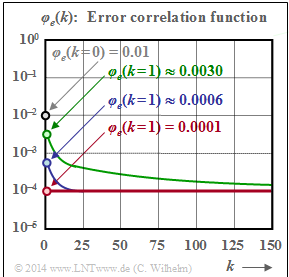
$\text{Example 9:}$ As in $\text{Example 8}$, $p_{\rm S} = 0.01$. The error correlation functions shown here again represent
- Green: $\alpha = 0.7$ ⇒ strong bursting.
- Blue: $\alpha = 0.95$ ⇒ weak bursting,
- Red: $\alpha = 1$ ⇒ BSC model.
The following statements can be generalized to a large extent, see also "GE model":
- The ECF value at the point $k = 0$ is equal to $p_{\rm S} = 10^{-2}$ for all channels (marked by the circle with gray filling) and the limit value for $k \to \infty$ is always $p_{\rm S}^2 = 10^{-4}$.
- In the BSC model, this final value is already reached at $k = 1$ (marked by a red filled circle). Here, therefore, the ECF can only assume the two values $p_{\rm S}$ and $p_{\rm S}^2$.
- Also for $\alpha < 1$ (blue and green curves), a fold can be seen at $k = 1$. After that, the ECF is monotonically decreasing. The decrease is the slower, the smaller $\alpha$ is, i.e. the more bursted the errors occur.
Analysis of error structures with the Wilhelm A model
Wilhelm developed his channel model mainly in order to be able to draw conclusions about the errors occurring from measured error sequences. From the multitude of analyses in [Wil11][5] only a few are to be quoted here, whereby always the symbol error probability $p_{\rm S} = 10^{-3}$ is the basis.
- In the diagrams, the red curve applies in each case to statistically independent errors $($BSC or $\alpha = 1)$,
- the green curve for a burst error channel with $\alpha = 0.7$. In addition, the following agreement shall apply:
$\text{Definition:}$ An error burst (or burst for short) always starts with a symbol error and ends when $k_{\rm Burst}- 1$ error-free symbols follow each other.
- $k_{\rm Burst}$ denotes the burst end parameter.
- The burst weight $G_{\rm Burst}$ corresponds to the number of all symbol errors in the burst.
- For a single error, gilt $G_{\rm Burst}= 1$ and the burst length (determined by the first and last error) is also $L_{\rm Burst}= 1$.
$\text{Example 10:}\ \text{Probability }p_1\text{ of a single error in a sample of length} \ n$
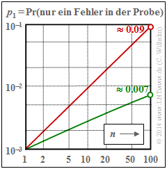
For the BSC channel $(\alpha = 1)$, $p_1 = n \cdot 0.001 \cdot 0.999^{n-1}$ ⇒ red curve. Due to the double-logarithmic representation, these numerical values result in a (nearly) linear progression. Thus, with the BSC model, single errors occur in a sample of length $n = 100$ with about $9\%$ probability.
In the case of the burst error channel with $\alpha = 0.7$ (green curve), the corresponding probability is only about $0.7\%$ and the course of the curve is slightly curved here.
In the following calculation, we first assume that the single error in the sample of length $n$ occurs at position $b$:
- In the case of a single error, $n-b$ error-free symbols must then follow. After averaging over the possible error positions $b$, we thus obtain:
- \[p_1 = p_{\rm S} \cdot \sum_{b = 1}^{n} \hspace{0.15cm}V_a (b) \cdot V_a (n+1-b) \hspace{0.05cm}.\]
- Because of its similarity to the signal representation of a "digital filter", the sum can be called a convolution of $V_a(b)$ with itself. For the generating function $V_a(z)$, the convolution becomes a product (or the square because of $V_a(b) \star V_a(b)$ ) and the following equation is obtained:
- \[V_a(z=1) \cdot V_a(z=1) = \big [ V_a(z=1) \big ]^2 = {\big [ 1 -(1- {p_{\rm S} }^{1/\alpha})\big ]^{-2\alpha} } \hspace{0.05cm}.\]
- Thus, with the "specific error distance distribution" $V_a(z)$, we obtain the following final result:
- \[p_1 = p_{\rm S} \cdot \frac{2\alpha \cdot (2\alpha+1) \cdot \hspace{0.05cm} \text{... } \hspace{0.05cm} \cdot (2\alpha+n-2)} {(n-1)!}\cdot (1- {p_{\rm S} }^{1/\alpha})^{n-1} \hspace{0.05cm}.\]
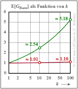
$\text{Example 11:}\ \text{Mean number of errors } {\rm E}[G_{\rm Burst}] \text{ in a burst with end parameter }k_{\rm Burst}$
Let the mean symbol error probability still be $p_{\rm S} = 10^{-3}$, i.e. (relatively) small.
(1) Red curve for the BSC channel (or $\alpha = 1)$:
- For example, the parameter $k_{\rm Burst}= 10$ means that the burst is finished when nine error-free symbols follow after one error. The probability for an error distance $a \le 9$ is extremely small when $p_{\rm S}$ is small $($hier: $10^{-3})$ äußerst klein. Daraus folgt weiter, dass dann (fast) jeder Einzelfehler als ein "Burst" aufgefasst wird, und es gilt ${\rm E}[G_{\rm Burst}] \approx 1.01$ .
- Bei größerem Burst–Endeparameter $k_{\rm Burst}$ nimmt auch die Wahrscheinlichkeit ${\rm Pr}(a \le k_{\rm Burst})$ deutlich zu und es kommt zu "Bursts" mit mehr als einem Fehler. Wählt man beispielsweise $k_{\rm Burst}= 100$, so beinhaltet ein "Burst" im Mittel $1.1$ Symbolfehler.
- Das bedeutet gleichzeitig, dass es auch beim BSC–Modell zu langen Fehlerbursts (entsprechend unserer Definition) kommen kann, wenn bei gegebenem $p_{\rm S}$ der Burst–Endeparameter zu groß gewählt ist oder bei vorgegebenem $k_{\rm Burst}$ die mittlere Fehlerwahrscheinlichkeit $p_{\rm S}$ zu groß ist.
(2) Grüne Kurve für den Wilhelm–Kanal mit $\alpha = 0.7$:
Das hier angegebene Verfahren zur numerischen Bestimmung der mittleren Fehleranzahl ${\rm E}[G_{\rm Burst}]$ eines Bursts kann unabhängig vom $\alpha$–Wert angewendet werden. Man geht wie folgt vor:
- Entsprechend den Fehlerabstandswahrscheinlichkeiten ${\rm Pr}(a=k)$ generiert man eine Fehlerfolge $e_1$, $e_2$, ... , $e_i$, ... mit den Fehlerabständen $a_1$, $a_2$, ... , $a_i$, ...
- Ist ein Fehlerabstand $a_i \ge k_{\rm Burst}$, so markiert dieser das Ende eines Bursts. Ein solches Ereignis tritt mit der Wahrscheinlichkeit ${\rm Pr}(a \ge k_{\rm Burst}) = V_a(k_{\rm Burst} )$ ein.
- Wir zählen solche Ereignisse "$a_i \ge k_{\rm Burst}$" im gesamten Block der Länge $n$. Deren Anzahl ist gleichzeitig die Anzahl $N_{\rm Burst}$ der Bursts im Block.
- Gleichzeitig gilt die Beziehung $N_{\rm Burst} = N_{\rm Fehler} \cdot V_a(k_{\rm Burst} )$, wobei $N_{\rm Fehler}$ die Anzahl aller Fehler im Block angibt.
- Daraus lässt sich die mittlere Fehlerzahl pro Burst in einfacher Weise berechnen:
- \[{\rm E}[G_{\rm Burst}] =\frac {N_{\rm Fehler} }{N_{\rm Burst} } =\frac {1}{V_a(k_{\rm Burst})}\hspace{0.05cm}.\]
Die Markierungen in der Grafik korrespondieren mit folgenden Zahlenwerten der Fehlerabstandsverteilung:
- Die grünen Kreise $($Wilhelm–Kanal, $\alpha = 0.7)$ ergeben sich aus $V_a(10) = 0.394$ und $V_a(100) = 0.193$.
- Die roten Kreise $($BSC–Kanal, $\alpha = 1)$ sind die Kehrwerte von $V_a(10) = 0.991$ und $V_a(100) = 0906$.
Aufgaben zum Kapitel
Aufgabe 5.6: Fehlerkorrelationsdauer
Aufgabe 5.6Z: GE-Modelleigenschaften
Aufgabe 5.7: McCullough-Parameter aus Gilbert-Elliott-Parameter
Aufgabe 5.7Z: Nochmals McCullough-Modell
Quellenverzeichnis
- ↑ Gilbert, E. N.: Capacity of Burst–Noise Channel. In: Bell Syst. Techn. J. Vol. 39, 1960, pp. 1253–1266.
- ↑ Elliott, E.O.: Estimates of Error Rates for Codes on Burst–Noise Channels. In: Bell Syst. Techn. J., Vol. 42, (1963), pp. 1977 – 1997.
- ↑ Huber, J.: Codierung für gedächtnisbehaftete Kanäle. Dissertation – Universität der Bundeswehr München, 1982.
- ↑ McCullough, R.H.: The Binary Regenerative Channel. In: Bell Syst. Techn. J. (47), 1968.
- ↑ 5.0 5.1 5.2 Wilhelm, C.: A-Model and L-Model, New Channel Models with Formulas for Probabilities of Error Structures. Neue Kanalmodelle mit Formeln für die Wahrscheinlichkeit von Fehlerstrukturen. Internet-Veröffentlichungen zu Channels-Networks, 2011ff.

