Difference between revisions of "Information Theory/Further Source Coding Methods"
| Line 163: | Line 163: | ||
| − | == | + | ==Burrows–Wheeler Transformation== |
<br> | <br> | ||
| − | + | To conclude this source coding chapter, we briefly discuss the algorithm published in 1994 by [https://en.wikipedia.org/wiki/Michael_Burrows Michael Burrows] and [https://en.wikipedia.org/wiki/David_Wheeler_(computer_scientist) David J. Wheeler] veröffentlichten Algorithmus [BW94]<ref>Burrows, M.; Wheeler, D.J.: ''A Block-sorting Lossless Data Compression Algorithm.'' Technical Report. Digital Equipment Corporation Communications, Palo Alto, 1994.</ref>, | |
| − | * | + | *which, although it has no compression potential on its own, |
| − | * | + | *but it greatly improves the compression capability of other methods. |
| − | [[File:P_ID2475__Inf_T_2_4_S3_neu.png|frame| | + | [[File:P_ID2475__Inf_T_2_4_S3_neu.png|frame|Example of the BWT (forward transformation)]] |
| − | <br> | + | <br>The Burrows–Wheeler Transformation accomplishes a blockwise sorting of data, which is illustrated in the diagram using the example of the text $\text{ANNAS_ANANAS}$ of length $N = 12$ : |
| − | * | + | *First, an eine $N×N$ matrix is generated from the string of length $N$ with each row resulting from the preceding row by cyclic left shift. |
| − | * | + | *Then the BWT matrix is sorted lexicographically. The result of the transformation is the last ⇒ $\text{L–Spalte}$ column. In the example, this results in $\text{_NSNNAANAAAS}$. |
| − | * | + | *Furthermore, the primary index $I$ must also be passed on. This indicates the row of the sorted BWT matrix that contains the original text (marked red in the graphic). |
| − | * | + | *Of course, no matrix operations are necessary to determine the $\text{L–column}$ and primary index. Rather, the BWT result can be found very quickly with pointer technology. |
<br clear=all> | <br clear=all> | ||
{{BlaueBox|TEXT= | {{BlaueBox|TEXT= | ||
| − | $\text{ | + | $\text{Furthermore, it should be noted about the BWT procedure:}$ |
| − | * | + | *Without an additional measure ⇒ a downstream „real compression” – the BWT does not lead to any data compression. |
| − | * | + | *Rather, there is even a slight increase in the amount of data, since in addition to the $N$ characters, the primary index $I$ now also be transmitted. |
| − | * | + | *For longer texts, however, this effect is negligible. Assuming 8 bit–ASCII–characters (one byte each)) and the block length $N = 256$ the number of bytes per block only increases from $256$ to $257$, , i.e. by only $0.4\%$.}} |
| − | + | We refer to the detailed descriptions of BWT in [Abel04]<ref>Abel, J.: ''Grundlagen des Burrows-Wheeler-Kompressionsalgorithmus''. In: Informatik Forschung & Entwicklung, no. 2, vol. 18, S. 80-87, Jan. 2004 </ref>. | |
| − | + | Finally, we will show how the original text can be reconstructed from the $\text{L–column}$ of the BWT matrix. | |
| − | * | + | * For this, one still needs the primary index $I$, as well as the first column of the BWT matrix. |
| − | * | + | *This $\text{F–column}$ (from „First”) does not have to be transferred, but results from the $\text{L–column}$ (from „Last”) very simply through lexicographic sorting. |
| − | [[File:P_ID2476__Inf_T_2_4_S3b_neu.png|frame| | + | [[File:P_ID2476__Inf_T_2_4_S3b_neu.png|frame|Example for BWT (back transformation)]] |
| − | <br> | + | <br>The graphic shows the procedure for the example under consideration: |
| − | * | + | *One starts in the line with the primary index $I$. The first character to be output is the $\rm A$ marked in red in the $\text{F–column}$ . This step is marked in the graphic with a yellow (1) . |
| − | * | + | *This $\rm A$ is the third $\rm A$ character in the $\text{F–column}$. Now look for the third $\rm A$ in the $\text{L–column}$, , find it in the line marked with '''(2)''' and output the corresponding '''N''' of the $\text{F–column}$ . |
| − | * | + | *The last '''N''' of the $\text{L–column}$ is found in line '''(3)'''. The character of the F column is output in the same line, i.e. an '''N''' again. |
| − | + | After $N = 12$ decoding steps, the reconstruction is completed. | |
<br clear=all> | <br clear=all> | ||
{{BlaueBox|TEXT= | {{BlaueBox|TEXT= | ||
| − | $\text{ | + | $\text{Conclusion:}$ |
| − | * | + | *This example has shown that the ''Burrows–Wheeler Transformation'' is nothing more than a sorting algorithm for texts. What is special about it is that the sorting is uniquely reversible. |
| − | * | + | *This property and additionally its inner structure are the basis for compressing the BWT result by means of known and efficient methods such as [[Information_Theory/Entropiecodierung_nach_Huffman|Huffman]] (a form of entropy coding) and [[Information_Theory/Weitere_Quellencodierverfahren#Run.E2.80.93Length_Coding|Run–Length Coding ]] .}} |
Revision as of 20:23, 29 March 2021
Contents
The Shannon-Fano algorithm
The Huffman coding from 1952 is a special case of „entropy coding”. It attempts to represent the source symbol $q_μ$ by a code symbol $c_μ$ of length $L_μ$ , aiming for the following construction rule:
- $$L_{\mu} \approx -{\rm log}_2\hspace{0.15cm}(p_{\mu}) \hspace{0.05cm}.$$
Since $L_μ$ , in contrast to $-{\rm log}_2\hspace{0.15cm}(p_{\mu})$ , is integer, this does not always succeed.
Already three years before David A. Huffman, Claude E. Shannon and Robert Fano gave a similar algorithm, namely:
- Order the source symbols according to decreasing probabilities of occurrence (identical to Huffman).
- Divide the sorted characters into two groups of equal probability.
- The binary symbol 1 is assigned to the first group, 0 to the second (or vice versa).
- If there is more than one character in a group, the algorithm is to be applied recursively to this group.
$\text{Example 1:}$ As in the introductory example for the Huffman algorithm in the last chapter, we assume $M = 6$ symbols and the following probabilities:
- $$p_{\rm A} = 0.30 \hspace{0.05cm},\hspace{0.2cm}p_{\rm B} = 0.24 \hspace{0.05cm},\hspace{0.2cm}p_{\rm C} = 0.20 \hspace{0.05cm},\hspace{0.2cm} p_{\rm D} = 0.12 \hspace{0.05cm},\hspace{0.2cm}p_{\rm E} = 0.10 \hspace{0.05cm},\hspace{0.2cm}p_{\rm F} = 0.04 \hspace{0.05cm}.$$
Then the Shannon-Fano algorithm is:
- $\rm AB$ → 1x (probability 0.54), $\rm CDEF$ → 0x (probability 0.46),
- $\underline{\rm A}$ → 11 (probability 0.30), $\underline{\rm B}$ → 10 (probability 0.24),
- $\underline{\rm C}$ → 01 (probability 0.20), $\rm DEF$ → 00x, (probability 0.26),
- $\underline{\rm D}$ → 001 (probability 0.12), $\rm EF$ → 000x (probability 0.14),
- $\underline{\rm E}$ → 0001 (probability 0.10), $\underline{\rm F}$ → 0000 (probability 0.04).
Notes:
- An „x” again indicates that bits must still be added in subsequent coding steps.
- This results in a different assignment than with Huffman coding, but exactly the same average codeword length: Huffman coding, but exactly the same average codeword length:
- $$L_{\rm M} = (0.30\hspace{-0.05cm}+\hspace{-0.05cm} 0.24\hspace{-0.05cm}+ \hspace{-0.05cm}0.20) \hspace{-0.05cm}\cdot\hspace{-0.05cm} 2 + 0.12\hspace{-0.05cm} \cdot \hspace{-0.05cm} 3 + (0.10\hspace{-0.05cm}+\hspace{-0.05cm}0.04) \hspace{-0.05cm}\cdot \hspace{-0.05cm}4 = 2.4\,{\rm bit/source symbol}\hspace{0.05cm}.$$
With the probabilities corresponding to $\text{example 1}$ , the Shannon-Fano algorithm leads to the same mean codeword length as Huffman coding. Similarly, for many (actually: most) other probability profiles, Huffman and Shannon-Fano are equivalent from an information-theoretic point of view.
However, there are definitely cases where the two methods differ in terms of (mean) codeword length, as the following example shows.
$\text{Example 2:}$ We consider $M = 5$ symbols with the following probabilities:
- $$p_{\rm A} = 0.38 \hspace{0.05cm}, \hspace{0.2cm}p_{\rm B}= 0.18 \hspace{0.05cm}, \hspace{0.2cm}p_{\rm C}= 0.16 \hspace{0.05cm},\hspace{0.2cm} p_{\rm D}= 0.15 \hspace{0.05cm}, \hspace{0.2cm}p_{\rm E}= 0.13 \hspace{0.3cm} \Rightarrow\hspace{0.3cm} H = 2.19\,{\rm bit/source symbol} \hspace{0.05cm}. $$
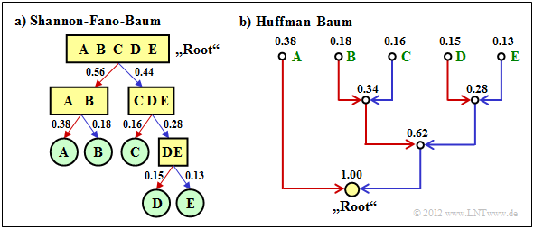
The diagram shows the respective code trees for Shannon-Fano (left) and Huffman (right). The results can be summarised as follows:
- The Shannon-Fano algorithm leads to the code $\rm A$ → 11, $\rm B$ → 10, $\rm C$ → 01, $\rm D$ → 001, $\rm E$ → 000 and thus to the mean code word length
- $$L_{\rm M} = (0.38 + 0.18 + 0.16) \cdot 2 + (0.15 + 0.13) \cdot 3 = 2.28\,\,{\rm bit/source symbol}\hspace{0.05cm}.$$
- Using „Huffman”, we get $\rm A$ → 1, $\rm B$ → 001, $\rm C$ → 010, $\rm D$ → 001, $\rm E$ → 000 and a slightly smaller mean codeword length:
- $$L_{\rm M} = 0.38 \cdot 1 + (1-0.38) \cdot 3 = 2.24\,\,{\rm bit/source symbol}\hspace{0.05cm}. $$
- There is no set of probabilities for which „Shannon–Fano” provides a better result than the Huffman algorithm, which always provides the best possible entropy encoder.
- The graph also shows that the algorithms proceed in different directions in the tree diagram, namely once from the root to the individual symbols (Shannon–Fano, and secondly from the individual symbols to the root (Huffman).
Arithmetic coding
Another form of entropy coding is arithmetic coding. Here, too, the symbol probabilities $p_μ$ must be known. For the index, $μ = 1$, ... , $M$.
Here is a brief outline of the procedure:
- In contrast to Huffman and Shannon-Fano coding, a symbol sequence of length $N$ is coded together in arithmetic coding. We write abbreviated $Q = 〈\hspace{0.05cm} q_1, q_2$, ... , $q_N \hspace{0.05cm} 〉$.
- Each symbol sequence $Q_i$ is assigned a real number interval $I_i$ which is identified by the beginning $B_i$ and the interval width ${\it Δ}_i$ .
- The „code” for the sequence $Q_i$ is the binary representation of a real number value from this interval: $r_i ∈ I_i = \big [B_i, B_i + {\it Δ}_i\big)$. This notation says that $B_i$ belongs to the interval $I_i$ (square bracket), but $B_i + {\it Δ}_i$ just does not (round bracket).
- It is always $0 ≤ r_i < 1$. It makes sense to select $r_i$ from the interval $I_i$ in such a way that the value can be represented with as few bits as possible. However, there is always a minimum number of bits, which depends on the interval width ${\it Δ}_i$ .
The algorithm for determining the interval parameters $B_i$ and ${\it Δ}_i$ is explained later in $\text{example 4}$ , as is a decoding option.
- First, there is a short example for the selection of the real number $r_i$ with regard to the minimum number of bits.
- More detailed information on this can be found in the description of task 2.11Z.
$\text{Example 3:}$ For the two parameter sets of the arithmetic coding algorithm listed below, the following real results $r_i$ and the following codes belong to the associated interval $I_i$ :
- $B_i = 0.25, {\it Δ}_i = 0.10 \ ⇒ \ I_i = \big[0.25, 0.35\big)\text{:}$
- $$r_i = 0 \cdot 2^{-1} + 1 \cdot 2^{-2} = 0.25 \hspace{0.3cm}\Rightarrow\hspace{0.3cm} {\rm Code} \hspace{0.15cm} \boldsymbol{\rm 01} \in I_i \hspace{0.05cm},$$
- $B_i = 0.65, {\it Δ}_i = 0.10 \ ⇒ \ I_i = \big[0.65, 0.75\big);$ note: $0.75$ does not belong to the interval:
- $$r_i = 1 \cdot 2^{-1} + 0 \cdot 2^{-2} + 1 \cdot 2^{-3} + 1 \cdot 2^{-4} = 0.6875 \hspace{0.3cm}\Rightarrow\hspace{0.3cm} {\rm Code} \hspace{0.15cm} \boldsymbol{\rm 1011} \in I_i\hspace{0.05cm}. $$
However, to organise the sequential flow, one chooses the number of bits constant to $N_{\rm Bit} = \big\lceil {\rm log}_2 \hspace{0.15cm} ({1}/{\it \Delta_i})\big\rceil+1\hspace{0.05cm}. $
- With the interval width ${\it Δ}_i = 0.10$ results $N_{\rm Bit} = 5$.
- So the actual arithmetic codes would be 01000 and 10110 respectively.
$\text{Example 4:}$ Now let the symbol range be $M = 3$ and let the symbols be denoted by $\rm X$, $\rm Y$ and $\rm Z$:
- The character sequence $\rm XXYXZ$ ⇒ length of the source symbol sequence: $N = 5$.
- Assume the probabilities $p_{\rm X} = 0.6$, $p_{\rm Y} = 0.2$ und $p_{\rm Z} = 0.2$.
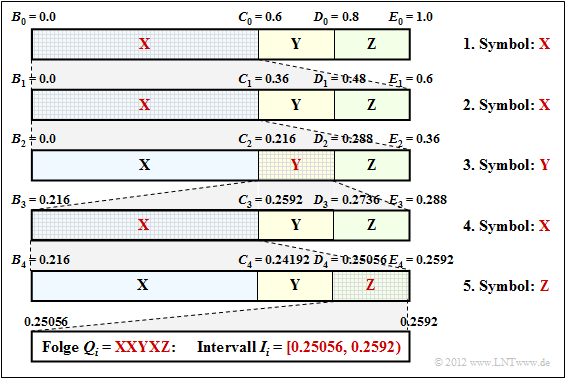
The diagram shows the algorithm for determining the interval boundaries.
- First, the entire probability range $($between $0$ and $1)$ is divided according to the symbol probabilities $p_{\rm X}$, $p_{\rm Y}$ and $p_{\rm Z}$ into three areas with the boundaries $B_0$, $C_0$, $D_0$ and $E_0$.
- The first symbol present for coding is $\rm X$. Therefore, in the next step, the probability range from $B_1 = B_0 = 0$ to $E_1 = C_0 = 0.6$ is again divided in the ratio $0.6$ : $0.2$ : $0.2$ .
- After the second symbol $\rm X$ , the range limits are $B_2 = 0$, $C_2 = 0.216$, $D_2 = 0.288$ and $E_2 = 0.36$. Since the symbol $\rm Y$ is now pending, the range is subdivided between $0.216$ ... $0.288$.
- After the fifth symbol $\rm Z$ , the interval $I_i$ for the considered symbol sequence $Q_i = \rm XXYXZ$ is fixed. A real number $r_i$ must now be found for which the following applies:: $0.25056 ≤ r_i < 0.2592$.
- The only real number in the interval $I_i = \big[0.25056, 0.2592\big)$, that can be represented with seven bits is $r_i = 1 · 2^{–2} + 1 · 2^{–7} = 0.2578125$. Thus the coder output is fixed: 0100001.
Seven bits are therefore needed for these $N = 5$ symbols, exactly as many as with Huffman coding with the assignment $\rm X$ → 1, $\rm Y$ → 00, $\rm Z$ → 01.
- However, arithmetic coding is superior to Huffman coding when the actual number of bits used in Huffman deviates even more from the optimal distribution, for example, when a character occurs extremely frequently.
- Often, however, only the middle of the interval – in the example $0.25488$ – is represented in binary: 0.01000010011 .... The number of bits is obtained as follows:
- $${\it Δ}_5 = 0.2592 - 0.25056 = 0.00864 \hspace{0.3cm}\Rightarrow \hspace{0.3cm}N_{\rm Bit} = \left\lceil {\rm log}_2 \hspace{0.15cm} \frac{1}{0.00864} \right\rceil + 1\hspace{0.15cm} = \left\lceil {\rm log}_2 \hspace{0.15cm} 115.7 \right\rceil + 1 = 8 \hspace{0.05cm}.$$
- Thus the arithmetic code for this example with $N = 5$ input characters is: 01000010.
- The decoding process can also be explained using the above graphic. The incoming bit sequence 0100001 wird zu $r = 0.2578125$ is converted to.
- This lies in the first and second step respectively in the first area ⇒ symbol $\rm X$, in the third step in the second area ⇒ symbol $\rm Y$, etc.
Further information on arithmetic coding can be found in WIKIPEDIA and in [BCK02][1].
Run–Length Coding
We consider a binary source $(M = 2)$ with the symbol set $\{$ $\rm A$, $\rm B$ $\}$, where one symbol occurs much more frequently than the other. For example, let $p_{\rm A} \gg p_{\rm B}$.
- Entropy coding only makes sense here when applied to $k$–tuples.
- A second possibility is Run-length coding (RLC), which considers the rarer character $\rm B$ as a separator and returns the lengths $L_i$ der einzelnen Substrings $\rm AA\text{...}A$ as a result.
$\text{Example 5:}$ The graphic shows an example sequence with the probabilities $p_{\rm A} = 0.9$ and $p_{\rm B} = 0.1$ ⇒ source entropy $H = 0.469$ bit/source symbol.
The example sequence of length $N = 100$ contains symbol $\rm B$ exactly ten times and symbol $\rm A$ ninety times, i.e. the relative frequencies here correspond exactly to the probabilities.
You can see from this example:
- The run length coding of this sequence results in the sequence $ \langle \hspace{0.05cm}6, \ 14, \ 26, \ 11, \ 4, \ 10, \ 3,\ 9,\ 1,\ 16 \hspace{0.05cm} \rangle $.
- If one represents the lengths $L_1$, ... , $L_{10}$ with five bits each, one thus requires $5 · 10 = 50$ Bit.
- The RLC–data compression is thus not much worse than the theoretical limit that results according to the source entropy to $H · N ≈ 47$ bits.
- The direct application of entropy coding would not result in any data compression here; rather, one continues to need $100$ bits.
- Even with the formation of triples, $54$ bits would still be needed with Huffman, i.e. more than with run-length coding.
However, the example also shows two problems of run-length coding:
- The lengths $L_i$ of the substrings are not limited. Special measures must be taken here if a length $L_i$ is greater than $2^5 = 32$ $($valid fo $N_{\rm Bit} = 5)$, for example the variant Run–Length Limited Coding (RLLC). See also [Meck09][2] and task 2.13.
- If the sequence does not end with $\rm B$ – which is rather the normal case with small probability $p_{\rm B}$ one must also provide special treatment for the end of the file.
Burrows–Wheeler Transformation
To conclude this source coding chapter, we briefly discuss the algorithm published in 1994 by Michael Burrows and David J. Wheeler veröffentlichten Algorithmus [BW94][3],
- which, although it has no compression potential on its own,
- but it greatly improves the compression capability of other methods.
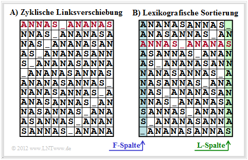
The Burrows–Wheeler Transformation accomplishes a blockwise sorting of data, which is illustrated in the diagram using the example of the text $\text{ANNAS_ANANAS}$ of length $N = 12$ :
- First, an eine $N×N$ matrix is generated from the string of length $N$ with each row resulting from the preceding row by cyclic left shift.
- Then the BWT matrix is sorted lexicographically. The result of the transformation is the last ⇒ $\text{L–Spalte}$ column. In the example, this results in $\text{_NSNNAANAAAS}$.
- Furthermore, the primary index $I$ must also be passed on. This indicates the row of the sorted BWT matrix that contains the original text (marked red in the graphic).
- Of course, no matrix operations are necessary to determine the $\text{L–column}$ and primary index. Rather, the BWT result can be found very quickly with pointer technology.
$\text{Furthermore, it should be noted about the BWT procedure:}$
- Without an additional measure ⇒ a downstream „real compression” – the BWT does not lead to any data compression.
- Rather, there is even a slight increase in the amount of data, since in addition to the $N$ characters, the primary index $I$ now also be transmitted.
- For longer texts, however, this effect is negligible. Assuming 8 bit–ASCII–characters (one byte each)) and the block length $N = 256$ the number of bytes per block only increases from $256$ to $257$, , i.e. by only $0.4\%$.
We refer to the detailed descriptions of BWT in [Abel04][4].
Finally, we will show how the original text can be reconstructed from the $\text{L–column}$ of the BWT matrix.
- For this, one still needs the primary index $I$, as well as the first column of the BWT matrix.
- This $\text{F–column}$ (from „First”) does not have to be transferred, but results from the $\text{L–column}$ (from „Last”) very simply through lexicographic sorting.
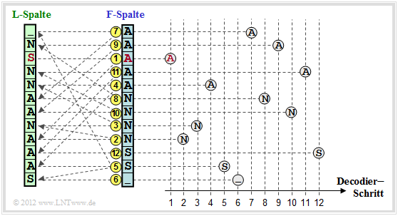
The graphic shows the procedure for the example under consideration:
- One starts in the line with the primary index $I$. The first character to be output is the $\rm A$ marked in red in the $\text{F–column}$ . This step is marked in the graphic with a yellow (1) .
- This $\rm A$ is the third $\rm A$ character in the $\text{F–column}$. Now look for the third $\rm A$ in the $\text{L–column}$, , find it in the line marked with (2) and output the corresponding N of the $\text{F–column}$ .
- The last N of the $\text{L–column}$ is found in line (3). The character of the F column is output in the same line, i.e. an N again.
After $N = 12$ decoding steps, the reconstruction is completed.
$\text{Conclusion:}$
- This example has shown that the Burrows–Wheeler Transformation is nothing more than a sorting algorithm for texts. What is special about it is that the sorting is uniquely reversible.
- This property and additionally its inner structure are the basis for compressing the BWT result by means of known and efficient methods such as Huffman (a form of entropy coding) and Run–Length Coding .
Anwendungsszenario für die Burrows–Wheeler–Transformation
Als Beispiel für die Einbettung der Burrows–Wheeler–Transformation (BWT) in eine Kette von Quellencodierverfahren wählen wir eine in [Abel03][5] vorgeschlagene Struktur. Wir verwenden dabei das gleiche Textbeispiel $\text{ANNAS_ANANAS}$ wie auf der letzten Seite. Die entsprechenden Strings nach den einzelnen Blöcken sind in der Grafik ebenfalls angegeben.
- Das BWT–Ergebnis lautet: $\text{_NSNNAANAAAS}$. An der Textlänge $N = 12$ hat die BWT nichts verändert, doch gibt es jetzt vier Zeichen, die identisch mit ihren Vorgängerzeichen sind (in der Grafik rot hervorgehoben). Im Originaltext war dies nur einmal der Fall.
- Im nächsten Block MTF (Move–To–Front) wird aus jedem Eingangszeichen aus der Menge $\{$ $\rm A$, $\rm N$, $\rm S$, _$\}$ ein Index $I ∈ \{0, 1, 2, 3\}$. Es handelt sich hierbei aber nicht um ein einfaches Mapping, sondern um einen Algorithmus, der in der Aufgabe 1.13Z angegeben ist.
- Für unser Beispiel lautet die MTF–Ausgangsfolge $323303011002$, ebenfalls mit der Länge $N = 12$. Die vier Nullen in der MTF–Folge (in der Grafik ebenfalls mit roter Schrift) geben an, dass an diesen Stellen das BWT–Zeichen jeweils gleich ist wie sein Vorgänger.
- Bei großen ASCII–Dateien kann die Häufigkeit der $0$ durchaus mehr als $50\%$ betragen, während die anderen $255$ Indizes nur selten auftreten. Zur Komprimierung einer solchen Textstruktur eignet sich eine Lauflängencodierung (englisch: Run–Length Coding, RLC) hervorragend.
- Der Block RLC0 in obiger Codierungskette bezeichnet eine spezielle Lauflängencodierung für Nullen. Die graue Schattierung der Nullen soll andeuten, dass hier eine lange Nullsequenz durch eine spezifische Bitfolge (kürzer als die Nullsequenz) maskiert wurde.
- Der Entropiecodierer $($EC, zum Beispiel „Huffman”$)$ sorgt für eine weitere Komprimierung. BWT und MTF haben in der Codierungskette nur die Aufgabe, durch eine Zeichenvorverarbeitung die Effizienz von RLC0 und EC zu steigern. Die Ausgangsdatei ist wieder binär.
Aufgaben zum Kapitel
Aufgabe 2.10: Shannon-Fano-Codierung
Aufgabe 2.11: Arithmetische Codierung
Aufgabe 2.11Z: Nochmals Arithmetische Codierung
Aufgabe 2.12: Run–Length Coding & RLLC
Aufgabe 2.13: Burrows-Wheeler-Rücktransformation
Aufgabe 2.13Z: Kombination BWT & „Move-to-Front”
Quellenverzeichnis
- ↑ Bodden, E.; Clasen, M.; Kneis, J.: Algebraische Kodierung. Proseminar, Lehrstuhl für Informatik IV, RWTH Aachen, 2002.
- ↑ Mecking, M.: Information Theory. Vorlesungsmanuskript, Lehrstuhl für Nachrichtentechnik, Technische Universität München, 2009.
- ↑ Burrows, M.; Wheeler, D.J.: A Block-sorting Lossless Data Compression Algorithm. Technical Report. Digital Equipment Corporation Communications, Palo Alto, 1994.
- ↑ Abel, J.: Grundlagen des Burrows-Wheeler-Kompressionsalgorithmus. In: Informatik Forschung & Entwicklung, no. 2, vol. 18, S. 80-87, Jan. 2004
- ↑ Abel, J.: Verlustlose Datenkompression auf Grundlage der Burrows-Wheeler-Transformation. In: PIK - Praxis der Informationsverarbeitung und Kommunikation, no. 3, vol. 26, S. 140-144, Sept. 2003.


