Difference between revisions of "Signal Representation/Fast Fourier Transform (FFT)"
| (45 intermediate revisions by 7 users not shown) | |||
| Line 1: | Line 1: | ||
{{LastPage}} | {{LastPage}} | ||
{{Header | {{Header | ||
| − | |Untermenü= | + | |Untermenü=Time and Frequency-Discrete Signal Representation |
| − | |Vorherige Seite= | + | |Vorherige Seite=Spectrum Analysis |
|Nächste Seite= | |Nächste Seite= | ||
}} | }} | ||
| − | == | + | ==Complexity of DFT and IDFT== |
| − | + | <br> | |
| − | + | A disadvantage of the direct calculation of the $($generally complex$)$ DFT sequences | |
| − | :$$ | + | :$$\langle \hspace{0.03cm}D(\mu)\hspace{0.03cm}\rangle \hspace{0.2cm}\bullet\!\!-\!\!\!-(N)\!-\!\!\!-\!\!\hspace{0.05cm}\circ\, \hspace{0.2cm} \langle \hspace{0.03cm}d(\nu)\hspace{0.03cm} \rangle$$ |
| − | + | according to the equations given in chapter [[Signal_Representation/Discrete_Fourier_Transform_(DFT)|»Discrete Fourier Transform»]] $\rm (DFT)$ is the large computational cost. | |
| + | |||
| + | We consider as an example the DFT, i.e. the calculation of the $D(\mu)$ coefficients from the $d(\nu)$ coefficients: | ||
| − | $$ | + | :$$N \cdot D(\mu) = \sum_{\nu = 0 }^{N-1} |
d(\nu) \cdot {w}^{\hspace{0.03cm}\nu \hspace{0.03cm} \cdot \hspace{0.05cm}\mu} | d(\nu) \cdot {w}^{\hspace{0.03cm}\nu \hspace{0.03cm} \cdot \hspace{0.05cm}\mu} | ||
| − | + | = | |
| − | d(0) \cdot w^{\hspace{0.03cm}0} + d(1) \cdot w^{\hspace{0.03cm}\mu}+ d(2) \cdot w^{\hspace{0.03cm}2\mu}+ ... + d(N-1) \cdot w^{\hspace{0.03cm}(N-1)\cdot \mu} | + | d(0) \cdot w^{\hspace{0.03cm}0} + d(1) \cdot w^{\hspace{0.03cm}\mu}+ d(2) \cdot w^{\hspace{0.03cm}2\mu}+\hspace{0.05cm}\text{ ...} \hspace{0.05cm}+ d(N-1) \cdot w^{\hspace{0.03cm}(N-1)\cdot \mu}.$$ |
| − | + | The computational effort required for this is to be estimated, assuming that the powers of the complex rotation factor $w = {\rm e}^{-{\rm j} \hspace{0.05cm}\cdot \hspace{0.05cm}2 \pi/N}$ already exist in real and imaginary part form in a lookup table. To calculate a single coefficient, one then needs $N-1$ complex multiplications and as many complex additions, observing: | |
| − | + | *Each complex addition requires two real additions: | |
| − | * | ||
:$$(R_1 + {\rm j} \cdot I_1) + (R_2 + {\rm j} \cdot I_2) = (R_1 + | :$$(R_1 + {\rm j} \cdot I_1) + (R_2 + {\rm j} \cdot I_2) = (R_1 + | ||
R_2) + {\rm j} \cdot (I_1 + I_2)\hspace{0.05cm}.$$ | R_2) + {\rm j} \cdot (I_1 + I_2)\hspace{0.05cm}.$$ | ||
| − | * | + | *Each complex multiplication requires four real multiplications and two real additions $($a subtraction is treated as an addition$)$: |
:$$(R_1 + {\rm j} \cdot I_1) (R_2 + {\rm j} \cdot I_2) = (R_1 \cdot | :$$(R_1 + {\rm j} \cdot I_1) (R_2 + {\rm j} \cdot I_2) = (R_1 \cdot | ||
R_2 - I_1 \cdot I_2) + {\rm j} \cdot (R_1 \cdot I_2 + R_2 \cdot | R_2 - I_1 \cdot I_2) + {\rm j} \cdot (R_1 \cdot I_2 + R_2 \cdot | ||
I_1)\hspace{0.05cm}.$$ | I_1)\hspace{0.05cm}.$$ | ||
| − | * | + | *Thus, the following number of real multiplications and the number of real additions are required to calculate all $N$ coefficients in total: |
| − | :$$M = 4 \cdot N \cdot (N-1), | + | :$$M = 4 \cdot N \cdot (N-1),$$ |
| + | :$$A = 2 \cdot N \cdot | ||
(N-1)+2 \cdot N \cdot (N-1)=M \hspace{0.05cm}.$$ | (N-1)+2 \cdot N \cdot (N-1)=M \hspace{0.05cm}.$$ | ||
| − | *In | + | *In today's computers, multiplications and additions/subtractions need about the same computing time. It is sufficient to consider the total number $\mathcal{O} = M + A$ of all operations: |
:$$\mathcal{O} = 8 \cdot N \cdot (N-1) \approx 8 \cdot N^2\hspace{0.05cm}.$$ | :$$\mathcal{O} = 8 \cdot N \cdot (N-1) \approx 8 \cdot N^2\hspace{0.05cm}.$$ | ||
| − | |||
| + | {{BlaueBox|TEXT= | ||
| + | $\text{Conclusion:}$ | ||
| + | *For a Discrete Fourier Transform $\rm (DFT)$ with $N = 1000$ one already needs almost eight million arithmetic operations. The same applies to an IDFT. | ||
| + | |||
| + | *With $N =16$ still $1920$ computational operations are required. | ||
| − | + | *If the parameter $N$ is a power to the base $2$, more computationally efficient algorithms can be applied. The multitude of such methods known from the literature are summarized under the collective term »'''Fast Fourier Transform'''« – abbreviated $\text{FFT}$. All these methods are based on the »superposition theorem« of the DFT.}} | |
| − | == | + | ==Superposition theorem of the DFT== |
| − | + | <br> | |
| − | + | The graph illustrates the so-called »superposition theorem« of the DFT using the example of» $N = 16$. Shown here is the transition from the time domain to the spectral domain, i.e. the calculation of the spectral domain coefficients from the time domain coefficients: $\langle \hspace{0.03cm}D(\mu)\hspace{0.03cm}\rangle \hspace{0.2cm}\bullet\!\!-\!\!\!-(N)\!-\!\!\!-\!\!\hspace{0.05cm}\circ\, \hspace{0.2cm} \langle \hspace{0.03cm} d(\nu) \hspace{0.03cm}\rangle.$ | |
| − | [[File: | + | [[File:EN_Sig_T_5_5_S2.png|right|frame|Superposition theorem of the DFT]] |
| − | + | The algorithm described thereby is characterized by the following steps: | |
| − | * | + | *The sequence $\langle \hspace{0.1cm}d(\nu)\hspace{0.1cm}\rangle$ of length $N$ is divided into two subsequences $\langle \hspace{0.03cm} d_1(\nu)\hspace{0.03cm}\rangle$ and $\langle \hspace{0.03cm} d_2(\nu)\hspace{0.03cm}\rangle$ each of half length $($highlighted in yellow and green respectively in the graphic$)$. With $0 \le \nu \lt N/2$ one thus obtains the sequence elements |
| − | :$$d_1(\nu) = d(2\nu), | + | :$$d_1(\nu) = d(2\nu), $$ |
| + | :$$d_2(\nu) = d(2\nu+1) | ||
\hspace{0.05cm}.$$ | \hspace{0.05cm}.$$ | ||
| − | * | + | *The initial sequences $\langle \hspace{0.03cm}D_1(\mu )\hspace{0.03cm}\rangle$ and $\langle \hspace{0.03cm}D_2(\mu )\hspace{0.03cm}\rangle$ of the two sub-blocks result from this each by its own DFT, but now only with half length $N/2 = 8$: |
| − | :$$\langle D_1(\mu) \rangle \hspace{0.2cm}\bullet\!\!-\!\!\!-(N/2)\!-\!\!\!-\!\!\hspace{0.05cm}\circ\, \hspace{0.2cm} \langle d_1(\nu) \rangle , \hspace{0. | + | :$$\langle \hspace{0.03cm}D_1(\mu) \hspace{0.03cm}\rangle \hspace{0.2cm}\bullet\!\!-\!\!\!-(N/2)\!-\!\!\!-\!\!\hspace{0.05cm}\circ\, \hspace{0.2cm} \langle \hspace{0.03cm}d_1(\nu) \hspace{0.03cm}\rangle , $$ |
| − | + | :$$ \langle \hspace{0.03cm}D_2(\mu)\hspace{0.03cm} \rangle \hspace{0.2cm}\bullet\!\!-\!\!\!-(N/2)\!-\!\!\!-\!\!\hspace{0.05cm}\circ\, \hspace{0.2cm} \langle \hspace{0.03cm}d_2(\nu) \hspace{0.03cm}\rangle \hspace{0.05cm}.$$ | |
| − | * | + | *The initial values $\langle \hspace{0.03cm} D_2(\mu )\hspace{0.03cm}\rangle$ of the lower (green) DFT $($with $0 \le \mu \lt N/2)$ are then changed in the block outlined in red by complex rotation factors with respect to phase: |
| − | :$$D_2(\mu) \hspace{0.3cm} \Rightarrow \hspace{0.3cm}D_2(\mu) \cdot w^{\hspace{0.04cm}\mu}, \hspace{0.2cm}{\rm | + | :$$D_2(\mu) \hspace{0.3cm} \Rightarrow \hspace{0.3cm}D_2(\mu) \cdot w^{\hspace{0.04cm}\mu}, \hspace{0.2cm}{\rm with}\hspace{0.1cm}w = |
{\rm e}^{-{\rm j} \hspace{0.05cm}\cdot \hspace{0.05cm}2 \pi/N} \hspace{0.05cm}.$$ | {\rm e}^{-{\rm j} \hspace{0.05cm}\cdot \hspace{0.05cm}2 \pi/N} \hspace{0.05cm}.$$ | ||
| − | * | + | *Each single »'''butterfly'''« in the blue bordered block $($in the middle of the graph$)$ yields two elements of the searched sequence by addition or subtraction. With $0 \le \mu \lt N/2$ applies: |
| − | :$$ | + | :$$D(\mu) = {1}/{2}\cdot \big[D_1(\mu) + D_2(\mu) \cdot w^{\hspace{0.04cm}\mu}\big],$$ |
| − | + | :$$D(\mu +{N}/{2}) = {1}/{2}\cdot \big[D_1(\mu) - D_2(\mu) \cdot w^{\hspace{0.04cm}\mu}\big]\hspace{0.05cm}.$$ | |
| − | + | ||
| + | '''This first application of the superposition theorem thus roughly halves the computational effort.''' | ||
{{GraueBox|TEXT= | {{GraueBox|TEXT= | ||
| − | $\text{ | + | $\text{Example 1:}$ |
| − | + | Let the DFT coefficients $d(\nu)$ for the description of the time course be "triangular" according to '''line 2''' of the following table. Note here the periodic continuation of the DFT, so that the linear increase for $t \lt 0$ is given by the coefficients $d(8), \hspace{0.05cm}\text{ ...} \hspace{0.05cm}, d(15)$. | |
| − | + | Applying the DFT algorithm with $N = 16$ one obtains the spectral coefficients $D(\mu )$ given in '''line 3''' which would be equal $D(\mu ) = 4 \cdot \text{sinc}^2(\mu/2)$ if the aliasing error were neglected. We can see that the aliasing error only affects the odd coefficients $($shaded boxes$)$. For example, $D(1) = 16/ \pi^2 \approx 1.621\neq 1.642$ should be. | |
| − | [[File:Sig_T_5_5_S2b_Version2.png| | + | [[File:Sig_T_5_5_S2b_Version2.png|right|frame|Result table for $\text{Example 1}$ for the superposition theorem of the DFT $($Note: "Zeile" ⇒ "row"$)$]] |
| − | + | If we split the total sequence $\langle \hspace{0.03cm}d(\nu)\hspace{0.03cm}\rangle$ into two subsequences such that the first subsequence $\langle \hspace{0.03cm}{d_1}'(\nu)\hspace{0.03cm}\rangle$ ⇒ yellow marked has only even coefficients $(\nu = 0, 2, \hspace{0.03cm}\text{ ...} \hspace{0.1cm}, N–2)$ and the second subsequence $\langle \hspace{0.03cm}{d_2}'(\nu)\hspace{0.03cm}\rangle$ ⇒ green marked contains only odd coefficients $(\nu = 1, 3, \hspace{0.03cm}\text{ ...} \hspace{0.1cm} , N-1)$ and all others are set to zero. The corresponding sequences in the spectral domain are obtained: | |
| − | :$$ \langle {D_1}'(\mu) \rangle \hspace{0.2cm}\bullet\!\!-\!\!\!-(N)\!-\!\!\!-\!\!\hspace{0.05cm}\circ\, \hspace{0.2cm} \langle {d_1}'(\nu) \rangle , \hspace{0. | + | :$$ \langle \hspace{0.03cm}{D_1}'(\mu)\hspace{0.03cm} \rangle \hspace{0.2cm}\bullet\!\!-\!\!\!-(N)\!-\!\!\!-\!\!\hspace{0.05cm}\circ\, \hspace{0.2cm} \langle \hspace{0.03cm} {d_1}'(\nu) \hspace{0.03cm}\rangle , $$ |
| − | + | :$$ \langle \hspace{0.03cm}{D_2}'(\mu) \hspace{0.03cm}\rangle \hspace{0.2cm}\bullet\!\!-\!\!\!-(N)\!-\!\!\!-\!\!\hspace{0.05cm}\circ\, \hspace{0.2cm} \langle\hspace{0.03cm} {d_2}'(\nu) \rangle \hspace{0.03cm}\hspace{0.05cm}.$$ | |
| − | In | + | In the yellow or green lines $4\hspace{0.05cm}\text{ ...} \hspace{0.05cm}7$ you can see: |
| − | * | + | *Because of $d(\nu) = {d_1}'(\nu) + {d_2}'(\nu)$ also holds |
| − | * | + | :$$D(\mu ) = {D_1}'(\mu ) + {D_2}'(\mu ).$$ |
| + | :This can be justified, for example, with the [[Signal_Representation/Fourier_Transform_Theorems#Multiplication_with_a_factor_-_Addition_Theorem|»Addition Theorem of Linear Systems«]]. | ||
| + | *The period of the sequence $\langle \hspace{0.03cm}{D_1}'(\mu )\hspace{0.03cm}\rangle$ due to the zeroing of every second time coefficient is now $N/2$ unlike the period $N$ of the sequence $\langle \hspace{0.03cm} D(\mu )\hspace{0.03cm}\rangle$: | ||
:$${D_1}'(\mu + {N}/{2}) ={D_1}'(\mu)\hspace{0.05cm}.$$ | :$${D_1}'(\mu + {N}/{2}) ={D_1}'(\mu)\hspace{0.05cm}.$$ | ||
| − | * $\langle {D_2}'(\mu )\rangle$ | + | * The sequence $\langle \hspace{0.03cm} {D_2}'(\mu )\hspace{0.03cm}\rangle$ additionally contains a phase factor $($shift by one sample$)$ which causes a sign change of two coefficients separated by $N/2$: |
| − | :$${D_2}'(\mu + {N}/{2}) =-{D_2}'(\mu)\hspace{0.05cm}.$$ | + | :$${D_2}'(\mu + {N}/{2}) = - {D_2}'(\mu)\hspace{0.05cm}.$$ |
| − | * | + | *The calculation of $\langle \hspace{0.03cm}{D_1}'(\mu )\hspace{0.03cm}\rangle$ and $\langle \hspace{0.03cm} {D_2}'(\mu )\hspace{0.1cm}\rangle$ is, however, in each case as time-consuming as the determination of $\langle \hspace{0.03cm}D(\mu )\hspace{0.03cm}\rangle$, since $\langle \hspace{0.03cm}{d_1}'(\nu)\hspace{0.03cm}\rangle$ and $\langle \hspace{0.03cm}{d_2}'(\nu)\hspace{0.03cm}\rangle$ also consist of $N$ elements, even if half of them are zeros.}} |
| − | + | {{GraueBox|TEXT= | |
| + | $\text{Example 2:}$ | ||
| + | To continue the first example, the previous table is now extended by the rows $8$ to $12$ . | ||
| − | [[File: | + | [[File:EN_Sig_T_5_5_S2c.png|right|frame|Result table for $\text{Example 2}$ for the superposition theorem of the DFT]] |
| + | |||
| + | Omitting the coefficients ${d_1}'(\nu) = 0$ with odd indices and ${d_2}'(\nu) = 0$ with even indices, we arrive at the subsequences $\langle \hspace{0.03cm}d_1(\nu)\hspace{0.03cm}\rangle$ and $\langle \hspace{0.03cm}d_2(\nu)\hspace{0.03cm}\rangle$ corresponding to lines $9$ and $11$. | ||
| + | |||
| + | You can see: | ||
| + | *The time sequences $\langle \hspace{0.03cm}{d_1}(\nu )\hspace{0.03cm}\rangle$ and $\langle \hspace{0.03cm}{d_2}(\nu )\hspace{0.03cm}\rangle$ exhibit as well as the corresponding spectral sequences $\langle \hspace{0.03cm}{D_1}(\mu )\hspace{0.03cm}\rangle$ and $\langle \hspace{0.03cm}{D_2}(\mu )\hspace{0.03cm}\rangle$ only have the dimension $(N/2)$. | ||
| − | + | *A comparison of the lines $5$, $7$, $10$ and $12$ shows the following relationship for $0 \le \mu \lt N/2$ : | |
| − | + | :$${D_1}'(\mu) = {1}/{2}\cdot {D_1}(\mu)\hspace{0.05cm},$$ | |
| − | + | :$$ {D_2}'(\mu) = {1}/{2}\cdot {D_2}(\mu)\cdot w^{\hspace{0.04cm}\mu}\hspace{0.05cm}.$$ | |
| − | :$${D_1}'(\mu) = {1}/{2}\cdot {D_1}(\mu) | + | *Correspondingly, for $N/2 \le \mu \lt N$: |
| − | + | :$${D_1}'(\mu) = {1}/{2}\cdot {D_1}(\mu - {N}/{2})\hspace{0.05cm},$$ | |
| − | * | + | :$$ {D_2}'(\mu) = {1}/{2}\cdot {D_2}(\mu {-} {N}/{2})\cdot w^{\hspace{0.04cm}\mu}$$ |
| − | :$$ | + | :$$ \Rightarrow \hspace{0.3cm}{D_2}'(\mu) = { - } {1}/{2}\cdot {D_2}(\mu-N/2)\cdot w^{\hspace{0.04cm}\mu {-} N/2}\hspace{0.05cm}.$$ |
| − | + | ||
| − | + | *For example, with $N = 16$ ⇒ $w = {\rm e}^{ - {\rm j}\hspace{0.04cm} \cdot \hspace{0.04cm}\pi/8}$ for the indices $\mu = 1$ respectively $\mu = 9$: | |
| − | * | + | :$${D_1}'(1) = {1.708}/{2} = 0.854,\hspace{0.8cm} |
| − | :$${D_1}'(1) = {1.708}/{2} = 0.854,\hspace{0. | + | {D_2}'(1) ={1}/{2}\cdot (1.456 + {\rm j} 0.603) \cdot {\rm e}^{ - {\rm j} \hspace{0.05cm}\cdot \hspace{0.05cm} |
| − | {D_2}'(1) ={1}/{2}\cdot (1.456 + {\rm j} 0.603) \cdot {\rm e}^{-{\rm j} \hspace{0.05cm}\cdot \hspace{0.05cm} | ||
\pi/8} = 0.788$$ | \pi/8} = 0.788$$ | ||
:$$\Rightarrow D(1) = {D_1}'(1)+ {D_2}'(1)= 1.642 \hspace{0.05cm}.$$ | :$$\Rightarrow D(1) = {D_1}'(1)+ {D_2}'(1)= 1.642 \hspace{0.05cm}.$$ | ||
| − | :$${D_9}'(1) = {1.708}/{2} = 0.854,\hspace{0. | + | :$${D_9}'(1) = {1.708}/{2} = 0.854,\hspace{0.8cm} |
| − | + | {D_2}'(9) = - {1}/{2}\cdot (1.456 + {\rm j} 0.603) \cdot {\rm e}^{ - {\rm j} \hspace{0.05cm}\cdot \hspace{0.05cm} | |
| − | \pi/8} = -0.788$$ | + | \pi/8} = - 0.788$$ |
| − | :$$\Rightarrow D(9) = {D_1}'(9)+ {D_2}'(9)= 0.066 \hspace{0.05cm}.$$ | + | :$$\Rightarrow D(9) = {D_1}'(9)+ {D_2}'(9)= 0.066 \hspace{0.05cm}.$$}} |
| + | |||
| − | }} | + | {{BlaueBox|TEXT= |
| + | $\text{Conclusion:}$ | ||
| + | *This first application of the superposition theorem almost halves the computational effort. | ||
| + | |||
| + | *Instead of $\mathcal{O}= 1920$ one only needs $\mathcal{O} = 2 - 448 + 8 \cdot (4+2) + 16 \cdot 2 = 976$ real operations. | ||
| + | |||
| + | *The first summand accounts for the two DFT calculations with $N/2 = 8$. | ||
| + | *The remainder is needed for the eight complex multiplications and the $16$ complex additions and subtractions, respectively.}} | ||
| − | + | ==Radix-2 algorithm according to Cooley and Tukey== | |
| + | <br> | ||
| + | Like other FFT algorithms, the method [CT65]<ref name ='CT65'>Cooley, J.W.; Tukey, J.W.: An Algorithm for the Machine Calculation of Complex Fourier Series. <br>In: Mathematics of Computation, Vol. 19, No. 90. (Apr., 1965), pp. 297-301.</ref> from [https://en.wikipedia.org/wiki/James_Cooley »$\text{James W. Cooley}$«] and [https://en.wikipedia.org/wiki/John_Tukey »$\text{John W. Tukey}$«] is based on the superposition theorem of the DFT. It only works if the number of interpolation points is a power of two. | ||
| + | |||
| + | The diagram illustrates the algorithm for $N = 8$, again showing the transformation from the time to the frequency domain. | ||
| + | [[File:EN_Sig_T_5_5_S3a.png|right|frame|Radix-2 algorithm $($flow diagram$)$; note: "level" and stage" are synonymous terms]] | ||
| + | |||
| + | *Before the FFT algorithm, the input values $d(0), \hspace{0.05cm}\text{...} \hspace{0.1cm}, d( N - 1)$ have to be reordered in the grey block »Bit Reversal Operation«. | ||
| + | |||
| + | *The computation is done in $\text{log}_2 N = 3$ stages, where in each stage $N/2 = 4$ equal computations are performed with different $\mu$–values as exponent of the complex rotation factor. Such a basic operation is called »'''butterfly'''«. | ||
| − | + | *Each butterfly calculates from two $($generally complex$)$ input variables $A$ and $B$ the two output variables $A + B \cdot w^{\mu}$ and $A - B \cdot w^{\mu}$ according to the following sketch. | |
| − | |||
| − | |||
| − | [[File: | + | [[File:P_ID1174__Sig_T_5_5_S3b_neu.png|center|frame|Butterfly of the DFT algorithm]] |
| + | <br clear=all> | ||
| + | {{BlaueBox|TEXT= | ||
| + | $\text{Conclusion:}$ | ||
| + | The complex spectral coefficients $D(0), \hspace{0.05cm}\text{...} \hspace{0.1cm}, D( N - 1)$ are obtained at the output of the last stage after division by $N$. | ||
| + | *As shown in [[Aufgaben:Exercise_5.5Z:_Complexity_of_the_FFT|$\text{Exercise 5.5Z}$]], this results in a much shorter computation time compared to the DFT, for example for $N = 1024$ by more than a factor $150$. | ||
| − | + | *The inverse DFT for calculating the time coefficients from the spectral coefficients is done with the same algorithm and only slight modifications.}} | |
| − | * | ||
| − | |||
| − | |||
| − | + | {{GraueBox|TEXT= | |
| − | + | $\text{Example 3:}$ | |
| + | Finally, the C program $\text{fft(N, Re, Im)}$ according to the Radix-2 algorithm described above is given: | ||
| + | [[File:EN_Sig_Programm.png|right|frame|Radix-2 algorithm (C program)]] | ||
| + | *The two float arrays »Re« and »Im» contain the $N$ real and imaginary parts of the complex time coefficients $d(0)$, ... , $d( N - 1)$. | ||
| − | + | *In the same fields »Re« and »Im» the complex coefficients $D(0)$, ... , $D( N - 1)$ are returned to the main program. | |
| − | + | *Due to the »in-place programming«, $N$ complex storage elements are thus sufficient for this algorithm but only if the input values are reordered at the beginning. | |
| − | * | + | *This is done by the program »bit-reversal«, where the contents of ${\rm Re}( \nu)$ and ${\rm Im}( \nu)$ are entered into the elements ${\rm Re}( \kappa)$ and ${\rm Im}( \kappa)$. $\text{Example 4}$ illustrates this procedure.}} |
| − | + | <br clear=all> | |
| − | |||
| − | |||
| − | + | {{GraueBox|TEXT= | |
| + | [[File:EN_Sig_T_5_5_S3d_v2.png|100px|right|frame|Radix-2 algorithm $($Bit-reversal operation for $N = 8)$]] | ||
| + | $\text{Example 4: Bit-reversal operation}$ | ||
| − | + | #The new index $\kappa$ is obtained by writing the index $\nu$ as a dual number and then representing the $\text{log}_2 \hspace{0.05cm} N$ bits in reverse order.<br><br> | |
| + | #For example, $\nu = 3$ becomes the new index $\kappa = 6$.}} | ||
| − | == | + | ==Exercises for the chapter== |
| + | <br> | ||
| + | [[Aufgaben:Exercise 5.5: Fast Fourier Transform|Exercise 5.5: Fast Fourier Transform]] | ||
| − | [[Aufgaben:5. | + | [[Aufgaben:Exercise 5.5Z: Complexity of The FFT|Exercise 5.5Z: Complexity of the FFT]] |
| − | + | ==References== | |
Latest revision as of 16:38, 28 June 2023
Contents
Complexity of DFT and IDFT
A disadvantage of the direct calculation of the $($generally complex$)$ DFT sequences
- $$\langle \hspace{0.03cm}D(\mu)\hspace{0.03cm}\rangle \hspace{0.2cm}\bullet\!\!-\!\!\!-(N)\!-\!\!\!-\!\!\hspace{0.05cm}\circ\, \hspace{0.2cm} \langle \hspace{0.03cm}d(\nu)\hspace{0.03cm} \rangle$$
according to the equations given in chapter »Discrete Fourier Transform» $\rm (DFT)$ is the large computational cost.
We consider as an example the DFT, i.e. the calculation of the $D(\mu)$ coefficients from the $d(\nu)$ coefficients:
- $$N \cdot D(\mu) = \sum_{\nu = 0 }^{N-1} d(\nu) \cdot {w}^{\hspace{0.03cm}\nu \hspace{0.03cm} \cdot \hspace{0.05cm}\mu} = d(0) \cdot w^{\hspace{0.03cm}0} + d(1) \cdot w^{\hspace{0.03cm}\mu}+ d(2) \cdot w^{\hspace{0.03cm}2\mu}+\hspace{0.05cm}\text{ ...} \hspace{0.05cm}+ d(N-1) \cdot w^{\hspace{0.03cm}(N-1)\cdot \mu}.$$
The computational effort required for this is to be estimated, assuming that the powers of the complex rotation factor $w = {\rm e}^{-{\rm j} \hspace{0.05cm}\cdot \hspace{0.05cm}2 \pi/N}$ already exist in real and imaginary part form in a lookup table. To calculate a single coefficient, one then needs $N-1$ complex multiplications and as many complex additions, observing:
- Each complex addition requires two real additions:
- $$(R_1 + {\rm j} \cdot I_1) + (R_2 + {\rm j} \cdot I_2) = (R_1 + R_2) + {\rm j} \cdot (I_1 + I_2)\hspace{0.05cm}.$$
- Each complex multiplication requires four real multiplications and two real additions $($a subtraction is treated as an addition$)$:
- $$(R_1 + {\rm j} \cdot I_1) (R_2 + {\rm j} \cdot I_2) = (R_1 \cdot R_2 - I_1 \cdot I_2) + {\rm j} \cdot (R_1 \cdot I_2 + R_2 \cdot I_1)\hspace{0.05cm}.$$
- Thus, the following number of real multiplications and the number of real additions are required to calculate all $N$ coefficients in total:
- $$M = 4 \cdot N \cdot (N-1),$$
- $$A = 2 \cdot N \cdot (N-1)+2 \cdot N \cdot (N-1)=M \hspace{0.05cm}.$$
- In today's computers, multiplications and additions/subtractions need about the same computing time. It is sufficient to consider the total number $\mathcal{O} = M + A$ of all operations:
- $$\mathcal{O} = 8 \cdot N \cdot (N-1) \approx 8 \cdot N^2\hspace{0.05cm}.$$
$\text{Conclusion:}$
- For a Discrete Fourier Transform $\rm (DFT)$ with $N = 1000$ one already needs almost eight million arithmetic operations. The same applies to an IDFT.
- With $N =16$ still $1920$ computational operations are required.
- If the parameter $N$ is a power to the base $2$, more computationally efficient algorithms can be applied. The multitude of such methods known from the literature are summarized under the collective term »Fast Fourier Transform« – abbreviated $\text{FFT}$. All these methods are based on the »superposition theorem« of the DFT.
Superposition theorem of the DFT
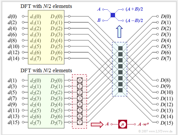
The graph illustrates the so-called »superposition theorem« of the DFT using the example of» $N = 16$. Shown here is the transition from the time domain to the spectral domain, i.e. the calculation of the spectral domain coefficients from the time domain coefficients: $\langle \hspace{0.03cm}D(\mu)\hspace{0.03cm}\rangle \hspace{0.2cm}\bullet\!\!-\!\!\!-(N)\!-\!\!\!-\!\!\hspace{0.05cm}\circ\, \hspace{0.2cm} \langle \hspace{0.03cm} d(\nu) \hspace{0.03cm}\rangle.$
The algorithm described thereby is characterized by the following steps:
- The sequence $\langle \hspace{0.1cm}d(\nu)\hspace{0.1cm}\rangle$ of length $N$ is divided into two subsequences $\langle \hspace{0.03cm} d_1(\nu)\hspace{0.03cm}\rangle$ and $\langle \hspace{0.03cm} d_2(\nu)\hspace{0.03cm}\rangle$ each of half length $($highlighted in yellow and green respectively in the graphic$)$. With $0 \le \nu \lt N/2$ one thus obtains the sequence elements
- $$d_1(\nu) = d(2\nu), $$
- $$d_2(\nu) = d(2\nu+1) \hspace{0.05cm}.$$
- The initial sequences $\langle \hspace{0.03cm}D_1(\mu )\hspace{0.03cm}\rangle$ and $\langle \hspace{0.03cm}D_2(\mu )\hspace{0.03cm}\rangle$ of the two sub-blocks result from this each by its own DFT, but now only with half length $N/2 = 8$:
- $$\langle \hspace{0.03cm}D_1(\mu) \hspace{0.03cm}\rangle \hspace{0.2cm}\bullet\!\!-\!\!\!-(N/2)\!-\!\!\!-\!\!\hspace{0.05cm}\circ\, \hspace{0.2cm} \langle \hspace{0.03cm}d_1(\nu) \hspace{0.03cm}\rangle , $$
- $$ \langle \hspace{0.03cm}D_2(\mu)\hspace{0.03cm} \rangle \hspace{0.2cm}\bullet\!\!-\!\!\!-(N/2)\!-\!\!\!-\!\!\hspace{0.05cm}\circ\, \hspace{0.2cm} \langle \hspace{0.03cm}d_2(\nu) \hspace{0.03cm}\rangle \hspace{0.05cm}.$$
- The initial values $\langle \hspace{0.03cm} D_2(\mu )\hspace{0.03cm}\rangle$ of the lower (green) DFT $($with $0 \le \mu \lt N/2)$ are then changed in the block outlined in red by complex rotation factors with respect to phase:
- $$D_2(\mu) \hspace{0.3cm} \Rightarrow \hspace{0.3cm}D_2(\mu) \cdot w^{\hspace{0.04cm}\mu}, \hspace{0.2cm}{\rm with}\hspace{0.1cm}w = {\rm e}^{-{\rm j} \hspace{0.05cm}\cdot \hspace{0.05cm}2 \pi/N} \hspace{0.05cm}.$$
- Each single »butterfly« in the blue bordered block $($in the middle of the graph$)$ yields two elements of the searched sequence by addition or subtraction. With $0 \le \mu \lt N/2$ applies:
- $$D(\mu) = {1}/{2}\cdot \big[D_1(\mu) + D_2(\mu) \cdot w^{\hspace{0.04cm}\mu}\big],$$
- $$D(\mu +{N}/{2}) = {1}/{2}\cdot \big[D_1(\mu) - D_2(\mu) \cdot w^{\hspace{0.04cm}\mu}\big]\hspace{0.05cm}.$$
This first application of the superposition theorem thus roughly halves the computational effort.
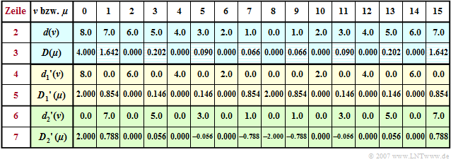
$\text{Example 1:}$ Let the DFT coefficients $d(\nu)$ for the description of the time course be "triangular" according to line 2 of the following table. Note here the periodic continuation of the DFT, so that the linear increase for $t \lt 0$ is given by the coefficients $d(8), \hspace{0.05cm}\text{ ...} \hspace{0.05cm}, d(15)$.
Applying the DFT algorithm with $N = 16$ one obtains the spectral coefficients $D(\mu )$ given in line 3 which would be equal $D(\mu ) = 4 \cdot \text{sinc}^2(\mu/2)$ if the aliasing error were neglected. We can see that the aliasing error only affects the odd coefficients $($shaded boxes$)$. For example, $D(1) = 16/ \pi^2 \approx 1.621\neq 1.642$ should be.
If we split the total sequence $\langle \hspace{0.03cm}d(\nu)\hspace{0.03cm}\rangle$ into two subsequences such that the first subsequence $\langle \hspace{0.03cm}{d_1}'(\nu)\hspace{0.03cm}\rangle$ ⇒ yellow marked has only even coefficients $(\nu = 0, 2, \hspace{0.03cm}\text{ ...} \hspace{0.1cm}, N–2)$ and the second subsequence $\langle \hspace{0.03cm}{d_2}'(\nu)\hspace{0.03cm}\rangle$ ⇒ green marked contains only odd coefficients $(\nu = 1, 3, \hspace{0.03cm}\text{ ...} \hspace{0.1cm} , N-1)$ and all others are set to zero. The corresponding sequences in the spectral domain are obtained:
- $$ \langle \hspace{0.03cm}{D_1}'(\mu)\hspace{0.03cm} \rangle \hspace{0.2cm}\bullet\!\!-\!\!\!-(N)\!-\!\!\!-\!\!\hspace{0.05cm}\circ\, \hspace{0.2cm} \langle \hspace{0.03cm} {d_1}'(\nu) \hspace{0.03cm}\rangle , $$
- $$ \langle \hspace{0.03cm}{D_2}'(\mu) \hspace{0.03cm}\rangle \hspace{0.2cm}\bullet\!\!-\!\!\!-(N)\!-\!\!\!-\!\!\hspace{0.05cm}\circ\, \hspace{0.2cm} \langle\hspace{0.03cm} {d_2}'(\nu) \rangle \hspace{0.03cm}\hspace{0.05cm}.$$
In the yellow or green lines $4\hspace{0.05cm}\text{ ...} \hspace{0.05cm}7$ you can see:
- Because of $d(\nu) = {d_1}'(\nu) + {d_2}'(\nu)$ also holds
- $$D(\mu ) = {D_1}'(\mu ) + {D_2}'(\mu ).$$
- This can be justified, for example, with the »Addition Theorem of Linear Systems«.
- The period of the sequence $\langle \hspace{0.03cm}{D_1}'(\mu )\hspace{0.03cm}\rangle$ due to the zeroing of every second time coefficient is now $N/2$ unlike the period $N$ of the sequence $\langle \hspace{0.03cm} D(\mu )\hspace{0.03cm}\rangle$:
- $${D_1}'(\mu + {N}/{2}) ={D_1}'(\mu)\hspace{0.05cm}.$$
- The sequence $\langle \hspace{0.03cm} {D_2}'(\mu )\hspace{0.03cm}\rangle$ additionally contains a phase factor $($shift by one sample$)$ which causes a sign change of two coefficients separated by $N/2$:
- $${D_2}'(\mu + {N}/{2}) = - {D_2}'(\mu)\hspace{0.05cm}.$$
- The calculation of $\langle \hspace{0.03cm}{D_1}'(\mu )\hspace{0.03cm}\rangle$ and $\langle \hspace{0.03cm} {D_2}'(\mu )\hspace{0.1cm}\rangle$ is, however, in each case as time-consuming as the determination of $\langle \hspace{0.03cm}D(\mu )\hspace{0.03cm}\rangle$, since $\langle \hspace{0.03cm}{d_1}'(\nu)\hspace{0.03cm}\rangle$ and $\langle \hspace{0.03cm}{d_2}'(\nu)\hspace{0.03cm}\rangle$ also consist of $N$ elements, even if half of them are zeros.
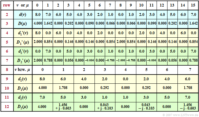
$\text{Example 2:}$ To continue the first example, the previous table is now extended by the rows $8$ to $12$ .
Omitting the coefficients ${d_1}'(\nu) = 0$ with odd indices and ${d_2}'(\nu) = 0$ with even indices, we arrive at the subsequences $\langle \hspace{0.03cm}d_1(\nu)\hspace{0.03cm}\rangle$ and $\langle \hspace{0.03cm}d_2(\nu)\hspace{0.03cm}\rangle$ corresponding to lines $9$ and $11$.
You can see:
- The time sequences $\langle \hspace{0.03cm}{d_1}(\nu )\hspace{0.03cm}\rangle$ and $\langle \hspace{0.03cm}{d_2}(\nu )\hspace{0.03cm}\rangle$ exhibit as well as the corresponding spectral sequences $\langle \hspace{0.03cm}{D_1}(\mu )\hspace{0.03cm}\rangle$ and $\langle \hspace{0.03cm}{D_2}(\mu )\hspace{0.03cm}\rangle$ only have the dimension $(N/2)$.
- A comparison of the lines $5$, $7$, $10$ and $12$ shows the following relationship for $0 \le \mu \lt N/2$ :
- $${D_1}'(\mu) = {1}/{2}\cdot {D_1}(\mu)\hspace{0.05cm},$$
- $$ {D_2}'(\mu) = {1}/{2}\cdot {D_2}(\mu)\cdot w^{\hspace{0.04cm}\mu}\hspace{0.05cm}.$$
- Correspondingly, for $N/2 \le \mu \lt N$:
- $${D_1}'(\mu) = {1}/{2}\cdot {D_1}(\mu - {N}/{2})\hspace{0.05cm},$$
- $$ {D_2}'(\mu) = {1}/{2}\cdot {D_2}(\mu {-} {N}/{2})\cdot w^{\hspace{0.04cm}\mu}$$
- $$ \Rightarrow \hspace{0.3cm}{D_2}'(\mu) = { - } {1}/{2}\cdot {D_2}(\mu-N/2)\cdot w^{\hspace{0.04cm}\mu {-} N/2}\hspace{0.05cm}.$$
- For example, with $N = 16$ ⇒ $w = {\rm e}^{ - {\rm j}\hspace{0.04cm} \cdot \hspace{0.04cm}\pi/8}$ for the indices $\mu = 1$ respectively $\mu = 9$:
- $${D_1}'(1) = {1.708}/{2} = 0.854,\hspace{0.8cm} {D_2}'(1) ={1}/{2}\cdot (1.456 + {\rm j} 0.603) \cdot {\rm e}^{ - {\rm j} \hspace{0.05cm}\cdot \hspace{0.05cm} \pi/8} = 0.788$$
- $$\Rightarrow D(1) = {D_1}'(1)+ {D_2}'(1)= 1.642 \hspace{0.05cm}.$$
- $${D_9}'(1) = {1.708}/{2} = 0.854,\hspace{0.8cm} {D_2}'(9) = - {1}/{2}\cdot (1.456 + {\rm j} 0.603) \cdot {\rm e}^{ - {\rm j} \hspace{0.05cm}\cdot \hspace{0.05cm} \pi/8} = - 0.788$$
- $$\Rightarrow D(9) = {D_1}'(9)+ {D_2}'(9)= 0.066 \hspace{0.05cm}.$$
$\text{Conclusion:}$
- This first application of the superposition theorem almost halves the computational effort.
- Instead of $\mathcal{O}= 1920$ one only needs $\mathcal{O} = 2 - 448 + 8 \cdot (4+2) + 16 \cdot 2 = 976$ real operations.
- The first summand accounts for the two DFT calculations with $N/2 = 8$.
- The remainder is needed for the eight complex multiplications and the $16$ complex additions and subtractions, respectively.
Radix-2 algorithm according to Cooley and Tukey
Like other FFT algorithms, the method [CT65][1] from »$\text{James W. Cooley}$« and »$\text{John W. Tukey}$« is based on the superposition theorem of the DFT. It only works if the number of interpolation points is a power of two.
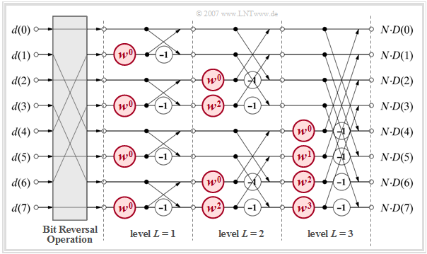
The diagram illustrates the algorithm for $N = 8$, again showing the transformation from the time to the frequency domain.
- Before the FFT algorithm, the input values $d(0), \hspace{0.05cm}\text{...} \hspace{0.1cm}, d( N - 1)$ have to be reordered in the grey block »Bit Reversal Operation«.
- The computation is done in $\text{log}_2 N = 3$ stages, where in each stage $N/2 = 4$ equal computations are performed with different $\mu$–values as exponent of the complex rotation factor. Such a basic operation is called »butterfly«.
- Each butterfly calculates from two $($generally complex$)$ input variables $A$ and $B$ the two output variables $A + B \cdot w^{\mu}$ and $A - B \cdot w^{\mu}$ according to the following sketch.
$\text{Conclusion:}$ The complex spectral coefficients $D(0), \hspace{0.05cm}\text{...} \hspace{0.1cm}, D( N - 1)$ are obtained at the output of the last stage after division by $N$.
- As shown in $\text{Exercise 5.5Z}$, this results in a much shorter computation time compared to the DFT, for example for $N = 1024$ by more than a factor $150$.
- The inverse DFT for calculating the time coefficients from the spectral coefficients is done with the same algorithm and only slight modifications.
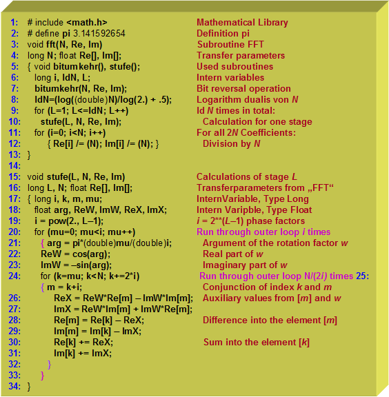
$\text{Example 3:}$ Finally, the C program $\text{fft(N, Re, Im)}$ according to the Radix-2 algorithm described above is given:
- The two float arrays »Re« and »Im» contain the $N$ real and imaginary parts of the complex time coefficients $d(0)$, ... , $d( N - 1)$.
- In the same fields »Re« and »Im» the complex coefficients $D(0)$, ... , $D( N - 1)$ are returned to the main program.
- Due to the »in-place programming«, $N$ complex storage elements are thus sufficient for this algorithm but only if the input values are reordered at the beginning.
- This is done by the program »bit-reversal«, where the contents of ${\rm Re}( \nu)$ and ${\rm Im}( \nu)$ are entered into the elements ${\rm Re}( \kappa)$ and ${\rm Im}( \kappa)$. $\text{Example 4}$ illustrates this procedure.
$\text{Example 4: Bit-reversal operation}$
- The new index $\kappa$ is obtained by writing the index $\nu$ as a dual number and then representing the $\text{log}_2 \hspace{0.05cm} N$ bits in reverse order.
- For example, $\nu = 3$ becomes the new index $\kappa = 6$.
Exercises for the chapter
Exercise 5.5: Fast Fourier Transform
Exercise 5.5Z: Complexity of the FFT
References
- ↑ Cooley, J.W.; Tukey, J.W.: An Algorithm for the Machine Calculation of Complex Fourier Series.
In: Mathematics of Computation, Vol. 19, No. 90. (Apr., 1965), pp. 297-301.
