Different Entropy Measures of Two-Dimensional Random Variables

Definition of entropy using supp(P_XY)

We briefly summarize the results of the last chapter again, assuming the two-dimensional random variable $XY$ with the probability mass function $P_{XY}(X,\ Y)$ . At the same time we use the notation

$${\rm supp} (P_{XY}) = \big \{ \hspace{0.05cm}(x,\ y) \in XY \hspace{0.05cm}, \hspace{0.3cm} {\rm where} \hspace{0.15cm} P_{XY}(X,\ Y) \ne 0 \hspace{0.05cm} \big \} \hspace{0.05cm};$$

$\text{Summarizing the last chapter:}$ With this subset $\text{supp}(P_{XY}) ⊂ P_{XY}$, the following holds for

the »joint entropy« :

$$H(XY) = {\rm E}\hspace{-0.1cm} \left [ {\rm log}_2 \hspace{0.1cm} \frac{1}{P_{XY}(X, Y)}\right ] =\hspace{-0.2cm} \sum_{(x, y) \hspace{0.1cm}\in \hspace{0.1cm}{\rm supp} (P_{XY}\hspace{-0.05cm})} \hspace{-0.6cm} P_{XY}(x, y) \cdot {\rm log}_2 \hspace{0.1cm} \frac{1}{P_{XY}(x, y)} \hspace{0.05cm}.$$

the »entropies of the one-dimensional random variables« $X$ and $Y$:

$$H(X) = {\rm E}\hspace{-0.1cm} \left [ {\rm log}_2 \hspace{0.1cm} \frac{1}{P_{X}(X)}\right ] =\hspace{-0.2cm} \sum_{x \hspace{0.1cm}\in \hspace{0.1cm}{\rm supp} (P_{X})} \hspace{-0.2cm} P_{X}(x) \cdot {\rm log}_2 \hspace{0.1cm} \frac{1}{P_{X}(x)} \hspace{0.05cm},$$

$$H(Y) = {\rm E}\hspace{-0.1cm} \left [ {\rm log}_2 \hspace{0.1cm} \frac{1}{P_{Y}(Y)}\right ] =\hspace{-0.2cm} \sum_{y \hspace{0.1cm}\in \hspace{0.1cm}{\rm supp} (P_{Y})} \hspace{-0.2cm} P_{Y}(y) \cdot {\rm log}_2 \hspace{0.1cm} \frac{1}{P_{Y}(y)} \hspace{0.05cm}.$$

$\text{Example 1:}$ We refer again to the examples on the $\text{joint probability and joint entropy}$ in the last chapter.

For the two-dimensional probability mass function $P_{RB}(R, B)$ in $\text{Example 5}$ with the parameters

$R$ ⇒ points of the red cube,
$B$ ⇒ points of the blue cube,

the sets $P_{RB}$ and $\text{supp}(P_{RB})$ are identical. Here, all $6^2 = 36$ squares are occupied by non-zero values.

For the two-dimensional probability mass function $P_{RS}(R, S)$ in $\text{Example 6}$ with the parameters

$R$ ⇒ points of the red cube,
$S = R + B$ ⇒ sum of both cubes,

there are $6 · 11 = 66$ squares, many of which, however, are empty, i.e. stand for the probability "0" .

The subset $\text{supp}(P_{RS})$ , on the other hand, contains only the $36$ shaded squares with non-zero probabilities.
The entropy remains the same no matter whether one averages over all elements of $P_{RS}$ or only over the elements of $\text{supp}(P_{RS})$ since for $x → 0$ the limit is $x · \log_2 ({1}/{x}) = 0$.

Conditional probability and conditional entropy

In the book "Theory of Stochastic Signals" the following $\text{conditional probabilities}$ were given for the case of two events $X$ and $Y$ ⇒ »Bayes' theorem«:

$${\rm Pr} (X \hspace{-0.05cm}\mid \hspace{-0.05cm} Y) = \frac{{\rm Pr} (X \cap Y)}{{\rm Pr} (Y)} \hspace{0.05cm}, \hspace{0.5cm} {\rm Pr} (Y \hspace{-0.05cm}\mid \hspace{-0.05cm} X) = \frac{{\rm Pr} (X \cap Y)}{{\rm Pr} (X)} \hspace{0.05cm}.$$

Applied to probability mass functions, one thus obtains:

$$P_{\hspace{0.03cm}X \mid \hspace{0.03cm} Y} (X \hspace{-0.05cm}\mid \hspace{-0.05cm} Y) = \frac{P_{XY}(X, Y)}{P_{Y}(Y)} \hspace{0.05cm}, \hspace{0.5cm} P_{\hspace{0.03cm}Y \mid \hspace{0.03cm} X} (Y \hspace{-0.05cm}\mid \hspace{-0.05cm} X) = \frac{P_{XY}(X, Y)}{P_{X}(X)} \hspace{0.05cm}.$$

Analogous to the $\text{joint entropy}$ $H(XY)$ , the following entropy functions can be derived here:

$\text{Definitions:}$

The »conditional entropy« of the random variable $X$ under condition $Y$ is:

$$H(X \hspace{-0.05cm}\mid \hspace{-0.05cm} Y) = {\rm E} \hspace{-0.1cm}\left [ {\rm log}_2 \hspace{0.1cm}\frac{1}{P_{\hspace{0.03cm}X \mid \hspace{0.03cm} Y} (X \hspace{-0.05cm}\mid \hspace{-0.05cm} Y)}\right ] = \hspace{-0.2cm} \sum_{(x, y) \hspace{0.1cm}\in \hspace{0.1cm}{\rm supp} (P_{XY}\hspace{-0.08cm})} \hspace{-0.6cm} P_{XY}(x, y) \cdot {\rm log}_2 \hspace{0.1cm} \frac{1}{P_{\hspace{0.03cm}X \mid \hspace{0.03cm} Y} (x \hspace{-0.05cm}\mid \hspace{-0.05cm} y)}=\hspace{-0.2cm} \sum_{(x, y) \hspace{0.1cm}\in \hspace{0.1cm}{\rm supp} (P_{XY}\hspace{-0.08cm})} \hspace{-0.6cm} P_{XY}(x, y) \cdot {\rm log}_2 \hspace{0.1cm} \frac{P_{Y}(y)}{P_{XY}(x, y)} \hspace{0.05cm}.$$

Similarly, for the »second conditional entropy« we obtain:

$$H(Y \hspace{-0.1cm}\mid \hspace{-0.05cm} X) = {\rm E} \hspace{-0.1cm}\left [ {\rm log}_2 \hspace{0.1cm}\frac{1}{P_{\hspace{0.03cm}Y\hspace{0.03cm} \mid \hspace{0.01cm} X} (Y \hspace{-0.08cm}\mid \hspace{-0.05cm}X)}\right ] =\hspace{-0.2cm} \sum_{(x, y) \hspace{0.1cm}\in \hspace{0.1cm}{\rm supp} (P_{XY}\hspace{-0.08cm})} \hspace{-0.6cm} P_{XY}(x, y) \cdot {\rm log}_2 \hspace{0.1cm} \frac{1}{P_{\hspace{0.03cm}Y\hspace{-0.03cm} \mid \hspace{-0.01cm} X} (y \hspace{-0.05cm}\mid \hspace{-0.05cm} x)}=\hspace{-0.2cm} \sum_{(x, y) \hspace{0.1cm}\in \hspace{0.1cm}{\rm supp} (P_{XY}\hspace{-0.08cm})} \hspace{-0.6cm} P_{XY}(x, y) \cdot {\rm log}_2 \hspace{0.1cm} \frac{P_{X}(x)}{P_{XY}(x, y)} \hspace{0.05cm}.$$

In the argument of the logarithm function there is always a conditional probability function ⇒ $P_{X\hspace{0.03cm}| \hspace{0.03cm}Y}(·)$ or $P_{Y\hspace{0.03cm}|\hspace{0.03cm}X}(·)$ resp., while the joint probability ⇒ $P_{XY}(·)$ is needed for the expectation value formation.

For the conditional entropies, there are the following limitations:

Both $H(X|Y)$ and $H(Y|X)$ are always greater than or equal to zero. From $H(X|Y) = 0$ it follows directly $H(Y|X) = 0$.
Both are only possible for $\text{disjoint sets}$ $X$ and $Y$.
$H(X|Y) ≤ H(X)$ and $H(Y|X) ≤ H(Y)$ always apply. These statements are plausible if one realizes that one can also use "uncertainty" synonymously for "entropy". For: The uncertainty with respect to the quantity $X$ cannot be increased by knowing $Y$.
Except in the case of statistical independence ⇒ $H(X|Y) = H(X)$ , $H(X|Y) < H(X)$ always holds. Because of $H(X) ≤ H(XY)$ and $H(Y) ≤ H(XY)$ , therefore also $H(X|Y) ≤ H(XY)$ and $H(Y|X) ≤ H(XY)$ hold. Thus, a conditional entropy can never become larger than the joint entropy.

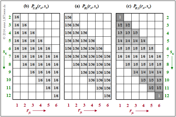
$\text{Example 2:}$ We consider the joint probabilities $P_{RS}(·)$ of our dice experiment, which were determined in the "last chapter" as $\text{Example 6}$. The corresponding $P_{RS}(·)$ is given again in the middle of the following graph.

Joint probabilities $P_{RS}$ and conditional probabilities $P_{S \vert R}$ and $P_{R \vert S}$

The two conditional probability functions are drawn on the outside:

$\text{On the left}$ you see the conditional probability mass function

$$P_{S \vert R}(⋅) = P_{SR}(⋅)/P_R(⋅).$$

Because of $P_R(R) = \big [1/6, \ 1/6, \ 1/6, \ 1/6, \ 1/6, \ 1/6 \big ]$ the probability $1/6$ is in all shaded fields
That means: $\text{supp}(P_{S\vert R}) = \text{supp}(P_{R\vert S})$ .
From this follows for the conditional entropy:

$$H(S \hspace{-0.1cm}\mid \hspace{-0.13cm} R) = \hspace{-0.2cm} \sum_{(r, s) \hspace{0.1cm}\in \hspace{0.1cm}{\rm supp} (P_{RS})} \hspace{-0.6cm} P_{RS}(r, s) \cdot {\rm log}_2 \hspace{0.1cm} \frac{1}{P_{\hspace{0.03cm}S \hspace{0.03cm} \mid \hspace{0.03cm} R} (s \hspace{-0.05cm}\mid \hspace{-0.05cm} r)} $$

$$\Rightarrow \hspace{0.3cm}H(S \hspace{-0.1cm}\mid \hspace{-0.13cm} R) = 36 \cdot \frac{1}{36} \cdot {\rm log}_2 \hspace{0.1cm} (6) = 2.585\ {\rm bit} \hspace{0.05cm}.$$

$\text{On the right}$, $P_{R\vert S}(⋅) = P_{RS}(⋅)/P_S(⋅)$ is given with $P_S(⋅)$ according to $\text{Example 6}$.

$\text{supp}(P_{R\vert S}) = \text{supp}(P_{S\vert R})$ ⇒ same non-zero fields result.
However, the probability values now increase continuously from the centre $(1/6)$ towards the edges up to $1$ in the corners.
It follows that:

$$H(R \hspace{-0.1cm}\mid \hspace{-0.13cm} S) = \frac{1}{36} \cdot {\rm log}_2 \hspace{0.1cm} (6) + \frac{2}{36} \cdot \sum_{i=1}^5 \big [ i \cdot {\rm log}_2 \hspace{0.1cm} (i) \big ]= 1.896\ {\rm bit} \hspace{0.05cm}.$$

On the other hand, for the conditional probabilities of the 2D random variable $RB$ according to $\text{Example 5}$, one obtains because of $P_{RB}(⋅) = P_R(⋅) · P_B(⋅)$:

$$\begin{align*}H(B \hspace{-0.1cm}\mid \hspace{-0.13cm} R) \hspace{-0.15cm} & = \hspace{-0.15cm} H(B) = {\rm log}_2 \hspace{0.1cm} (6) = 2.585\ {\rm bit} \hspace{0.05cm},\\ H(R \hspace{-0.1cm}\mid \hspace{-0.13cm} B) \hspace{-0.15cm} & = \hspace{-0.15cm} H(R) = {\rm log}_2 \hspace{0.1cm} (6) = 2.585\ {\rm bit} \hspace{0.05cm}.\end{align*}$$

Mutual information between two random variables

We consider the two-dimensional random variable $XY$ with PMF $P_{XY}(X, Y)$. Let the one-dimensional functions $P_X(X)$ and $P_Y(Y)$ also be known.

Now the following questions arise:

How does the knowledge of the random variable $Y$ reduce the uncertainty with respect to $X$?
How does the knowledge of the random variable $X$ reduce the uncertainty with respect to $Y$?

To answer this question, we need a definition that is substantial for information theory:

$\text{Definition:}$ The »mutual information« between the random variables $X$ and $Y$ – both over the same alphabet – is given as follows:

$$I(X;\ Y) = {\rm E} \hspace{-0.1cm}\left [ {\rm log}_2 \hspace{0.08cm} \frac{P_{XY}(X, Y)} {P_{X}(X) \cdot P_{Y}(Y) }\right ] =\hspace{-0.25cm} \sum_{(x, y) \hspace{0.1cm}\in \hspace{0.1cm}{\rm supp} (P_{XY})} \hspace{-0.8cm} P_{XY}(x, y) \cdot {\rm log}_2 \hspace{0.08cm} \frac{P_{XY}(x, y)} {P_{X}(x) \cdot P_{Y}(y) } \hspace{0.01cm}.$$

A comparison with the "last chapter" shows that the mutual information can also be written as a $\text{Kullback–Leibler distance}$ between the two-dimensional probability mass function $P_{XY}$ and the product $P_X · P_Y$ :

$$I(X;Y) = D(P_{XY} \hspace{0.05cm}\vert \vert \hspace{0.05cm} P_X \cdot P_Y) \hspace{0.05cm}.$$

It is thus obvious that $I(X;\ Y) ≥ 0$ always holds. Because of the symmetry, $I(Y;\ X)$ = $I(X;\ Y)$ is also true.

By splitting the $\log_2$ argument according to

$$I(X;Y) = {\rm E} \hspace{-0.1cm}\left [ {\rm log}_2 \hspace{0.1cm} \frac{1} {P_{X}(X) }\right ] - {\rm E} \hspace{-0.1cm}\left [ {\rm log}_2 \hspace{0.1cm} \frac {P_{Y}(Y) }{P_{XY}(X, Y)} \right ] $$

is obtained using $P_{X|Y}(\cdot) = P_{XY}(\cdot)/P_Y(Y)$:

$$I(X;Y) = H(X) - H(X \hspace{-0.1cm}\mid \hspace{-0.1cm} Y) \hspace{0.05cm}.$$

This means: The uncertainty regarding the random quantity $X$ ⇒ entropy $H(X)$ decreases by the magnitude $H(X|Y)$ when $Y$ is known. The remainder is the mutual information $I(X; Y)$.
With a different splitting, one arrives at the result

$$I(X;Y) = H(Y) - H(Y \hspace{-0.1cm}\mid \hspace{-0.1cm} X) \hspace{0.05cm}.$$

Ergo: The mutual information $I(X; Y)$ is symmetrical ⇒ $X$ says just as much about $Y$ as $Y$ says about $X$ ⇒ "mutual". The semicolon indicates equality.

$\text{Conclusion:}$ Often the equations mentioned here are clarified by a diagram, as in the following examples.
From this you can see that the following equations also apply:

$$I(X;\ Y) = H(X) + H(Y) - H(XY) \hspace{0.05cm},$$

$$I(X;\ Y) = H(XY) - H(X \hspace{-0.1cm}\mid \hspace{-0.1cm} Y) - H(Y \hspace{-0.1cm}\mid \hspace{-0.1cm} X) \hspace{0.05cm}.$$

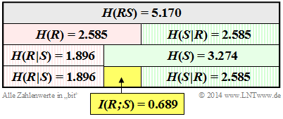
$\text{Example 3:}$ We return (for the last time) to the $\text{dice experiment}$ with the red $(R)$ and blue $(B)$ cube. The random variable $S$ gives the sum of the two dice: $S = R + B$. Here we consider the 2D random variable $RS$.

In earlier examples we calculated

the entropies $H(R) = 2.585 \ \rm bit$ and $H(S) = 3.274 \ \rm bit$ ⇒ $\text{Example 6}$ in the last chapter,
the join entropies $H(RS) = 5.170 \ \rm bit$ ⇒ $\text{Example 6}$ in the last chapter,
the conditional entropies $H(S \hspace{0.05cm} \vert \hspace{0.05cm} R) = 2.585 \ \rm bit$ and $H(R \hspace{0.05cm} \vert \hspace{0.05cm} S) = 1.896 \ \rm bit$ ⇒ $\text{Example 2}$ in the previous section.

Diagram of all entropies of the "dice experiment"

These quantities are compiled in the graph, with the random quantity $R$ marked by the basic colour "red" and the sum $S$ marked by the basic colour "green" . Conditional entropies are shaded. One can see from this representation:

The entropy $H(R) = \log_2 (6) = 2.585\ \rm bit$ is exactly half as large as the joint entropy $H(RS)$. Because: If one knows $R$, then $S$ provides exactly the same information as the random quantity $B$, namely $H(S \hspace{0.05cm} \vert \hspace{0.05cm} R) = H(B) = \log_2 (6) = 2.585\ \rm bit$.
Note: $H(R)$ = $H(S \hspace{0.05cm} \vert \hspace{0.05cm} R)$ only applies in this example, not in general.
As expected, here the entropy $H(S) = 3.274 \ \rm bit$ is greater than $H(R)= 2.585\ \rm bit$. Because of $H(S) + H(R \hspace{0.05cm} \vert \hspace{0.05cm} S) = H(R) + H(S \hspace{0.05cm} \vert \hspace{0.05cm} R)$ , $H(R \hspace{0.05cm} \vert \hspace{0.05cm} S)$ must therefore be smaller than $H(S \hspace{0.05cm} \vert \hspace{0.05cm} R)$ by $I(R;\ S) = 0.689 \ \rm bit$ . $H(R)$ is also smaller than $H(S)$ by $I(R;\ S) = 0.689 \ \rm bit$ .
The mutual information between the random variables $R$ and $S$ also results from the equation

$$I(R;\ S) = H(R) + H(S) - H(RS) = 2.585\ {\rm bit} + 3.274\ {\rm bit} - 5.170\ {\rm bit} = 0.689\ {\rm bit} \hspace{0.05cm}. $$

Conditional mutual information

We now consider three random variables $X$, $Y$ and $Z$, that can be related to each other.

$\text{Definition:}$ The »conditional mutual information« between the random variables $X$ and $Y$ for a given $Z = z$ is as follows:

$$I(X;Y \hspace{0.05cm}\vert\hspace{0.05cm} Z = z) = H(X\hspace{0.05cm}\vert\hspace{0.05cm} Z = z) - H(X\vert\hspace{0.05cm}Y ,\hspace{0.05cm} Z = z) \hspace{0.05cm}.$$

One denotes as the conditional »conditional mutual information« between the random variables $X$ and $Y$ for the random variable $Z$ in general
after averaging over all $z \in Z$:

$$I(X;Y \hspace{0.05cm}\vert\hspace{0.05cm} Z ) = H(X\hspace{0.05cm}\vert\hspace{0.05cm} Z ) - H(X\vert\hspace{0.05cm}Y Z )= \hspace{-0.3cm} \sum_{z \hspace{0.1cm}\in \hspace{0.1cm}{\rm supp} (P_{Z})} \hspace{-0.25cm} P_{Z}(z) \cdot I(X;Y \hspace{0.05cm}\vert\hspace{0.05cm} Z = z) \hspace{0.05cm}.$$

$P_Z(Z)$ is the probability mass function $\rm (PMF)$ of the random variable $Z$ and $P_Z(z)$ is the »probability« for the realization $Z = z$.

$\text{Please note:}$

For the conditional entropy, as is well known, the relation $H(X\hspace{0.05cm}\vert\hspace{0.05cm}Z) ≤ H(X)$ holds.
For the mutual information, this relation does not necessarily hold:
$I(X; Y\hspace{0.05cm}\vert\hspace{0.05cm}Z)$ can be smaller, equal, but also larger than $I(X; Y)$.

2D PMF $P_{XZ}$

$\text{Example 4:}$ We consider the binary random variables $X$, $Y$ and $Z$ with the following properties:

$X$ and $Y$ be statistically independent. Let the following be true for their probability mass functions:

$$P_X(X) = \big [1/2, \ 1/2 \big], \hspace{0.2cm} P_Y(Y) = \big[1– p, \ p \big] \ ⇒ \ H(X) = 1\ {\rm bit}, \hspace{0.2cm} H(Y) = H_{\rm bin}(p).$$

$Z$ is the modulo-2 sum of $X$ and $Y$: $Z = X ⊕ Y$.

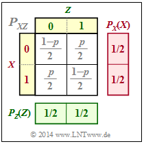
From the joint probability mass function $P_{XZ}$ according to the upper graph, it follows:

Summing the column probabilities gives
$P_Z(Z) = \big [1/2, \ 1/2 \big ]$ ⇒ $H(Z) = 1\ {\rm bit}.$
$X$ and $Z$ are also statistically independent, since for the 2D PMF holds
$P_{XZ}(X, Z) = P_X(X) · P_Z(Z)$ .

Conditional 2D PMF $P_{X\hspace{0.05cm}\vert\hspace{0.05cm}YZ}$

It follows that:
$H(Z\hspace{0.05cm}\vert\hspace{0.05cm} X) = H(Z),\hspace{0.5cm}(X \hspace{0.05cm}\vert\hspace{0.05cm} Z) = H(X),\hspace{0.5cm} I(X; Z) = 0.$

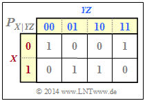
From the conditional probability mass function $P_{X\vert YZ}$ according to the graph below, we can calculate:

$H(X\hspace{0.05cm}\vert\hspace{0.05cm} YZ) = 0$, since all $P_{X\hspace{0.05cm}\vert\hspace{0.05cm} YZ}$ entries are $0$ or $1$ ⇒ "conditional entropy",
$I(X; YZ) = H(X) - H(X\hspace{0.05cm}\vert\hspace{0.05cm} YZ) = H(X)= 1 \ {\rm bit}$ ⇒ "mutual information",
$I(X; Y\vert Z) = H(X\hspace{0.05cm}\vert\hspace{0.05cm} Z) =H(X)=1 \ {\rm bit} $ ⇒ "conditional mutual information".

In the present example:

The conditional mutual information $I(X; Y\hspace{0.05cm}\vert\hspace{0.05cm} Z) = 1$ is greater than the conventional mutual information $I(X; Y) = 0$.

Chain rule of the mutual information

So far we have only considered the mutual information between two one-dimensional random variables. Now we extend the definition to a total of $n + 1$ random variables, which, only for reasons of representation, we denote with $X_1$, ... , $X_n$ and $Z$ . Then applies:

$\text{Chain rule of mutual information:}$

The mutual information between the $n$–dimensional random variable $X_1 X_2 \hspace{0.05cm}\text{...} \hspace{0.05cm} X_n$ and the random variable $Z$ can be represented and calculated as follows:

$$I(X_1\hspace{0.05cm}X_2\hspace{0.05cm}\text{...} \hspace{0.1cm}X_n;Z) = I(X_1;Z) + I(X_2;Z \vert X_1) + \hspace{0.05cm}\text{...} \hspace{0.1cm}+ I(X_n;Z\vert X_1\hspace{0.05cm}X_2\hspace{0.05cm}\text{...} \hspace{0.1cm}X_{n-1}) = \sum_{i = 1}^{n} I(X_i;Z \vert X_1\hspace{0.05cm}X_2\hspace{0.05cm}\text{...} \hspace{0.1cm}X_{i-1}) \hspace{0.05cm}.$$

$\text{Proof:}$ We restrict ourselves here to the case $n = 2$, i.e. to a total of three random variables, and replace $X_1$ by $X$ and $X_2$ by $Y$. Then we obtain:

$$\begin{align*}I(X\hspace{0.05cm}Y;Z) & = H(XY) - H(XY\hspace{0.05cm} \vert \hspace{0.05cm}Z) = \\ & = \big [ H(X)+ H(Y\hspace{0.05cm} \vert \hspace{0.05cm} X)\big ] - \big [ H(X\hspace{0.05cm} \vert \hspace{0.05cm} Z) + H(Y\hspace{0.05cm} \vert \hspace{0.05cm} XZ)\big ] =\\ & = \big [ H(X)- H(X\hspace{0.05cm} \vert \hspace{0.05cm} Z)\big ] - \big [ H(Y\hspace{0.05cm} \vert \hspace{0.05cm} X) + H(Y\hspace{0.05cm} \vert \hspace{0.05cm}XZ)\big ]=\\ & = I(X;Z) + I(Y;Z \hspace{0.05cm} \vert \hspace{0.05cm} X) \hspace{0.05cm}.\end{align*}$$

From this equation one can see that the relation $I(X Y; Z) ≥ I(X; Z)$ is always given.
Equality results for the conditional mutual information $I(Y; Z \hspace{0.05cm} \vert \hspace{0.05cm} X) = 0$, i.e. when the random variables $Y$ and $Z$ for a given $X$ are statistically independent.

$\text{Example 5:}$ We consider the $\text{Markov chain}$ $X → Y → Z$. For such a constellation, the "Data Processing Theorem" always holds with the following consequence, which can be derived from the chain rule of mutual information:

$$I(X;Z) \hspace{-0.05cm} \le \hspace{-0.05cm}I(X;Y ) \hspace{0.05cm},$$

$$I(X;Z) \hspace{-0.05cm} \le \hspace{-0.05cm} I(Y;Z ) \hspace{0.05cm}.$$

The theorem thus states:

One cannot gain any additional information about the input $X$ by manipulating the data $Y$ by processing $Y → Z$.
Data processing $Y → Z$ $($by a second processor$)$ only serves the purpose of making the information about $X$ more visible.

For more information on the "Data Processing Theorem" see "Exercise 3.15".