Difference between revisions of "Digital Signal Transmission/Block Coding with 4B3T Codes"
| Line 74: | Line 74: | ||
Fourier transforming the ACF yields the power-spectral density ${\it \Phi}_a(f)$ of the amplitude coefficients corresponding to the following graph from [TS87]<ref>Tröndle, K.; Söder, G.: Optimization of Digital Transmission Systems. Boston – London: Artech House, 1987, ISBN: 0-89006-225-0.</ref>. The outlined PSD was determined for the FoMoT code, whose Markov diagram is shown above. The differences between the individual 4B3T codes are not particularly pronounced. Thus, for the MS43 code ${\rm E}\big [a_\nu^2 \big ] \approx 0.65$ and for the other two 4B3T codes (Jessop/Waters, MS43) ${\rm E}\big [a_\nu^2 \big ] \approx 0.69$. <br> | Fourier transforming the ACF yields the power-spectral density ${\it \Phi}_a(f)$ of the amplitude coefficients corresponding to the following graph from [TS87]<ref>Tröndle, K.; Söder, G.: Optimization of Digital Transmission Systems. Boston – London: Artech House, 1987, ISBN: 0-89006-225-0.</ref>. The outlined PSD was determined for the FoMoT code, whose Markov diagram is shown above. The differences between the individual 4B3T codes are not particularly pronounced. Thus, for the MS43 code ${\rm E}\big [a_\nu^2 \big ] \approx 0.65$ and for the other two 4B3T codes (Jessop/Waters, MS43) ${\rm E}\big [a_\nu^2 \big ] \approx 0.69$. <br> | ||
| + | The statements of this graph can be summarized as follows: | ||
| + | |||
[[File:P_ID1336__Dig_T_2_3_S3b_v1.png|right|frame|Power-spectral density (of amplitude coefficients) of 4B3T compared to redundancy-free and AMI coding '''Korrektur'''|class=fit]] | [[File:P_ID1336__Dig_T_2_3_S3b_v1.png|right|frame|Power-spectral density (of amplitude coefficients) of 4B3T compared to redundancy-free and AMI coding '''Korrektur'''|class=fit]] | ||
| − | |||
*The graph shows the power-spectral density ${\it \Phi}_a(f)$ of the amplitude coefficients $a_\nu$ of the 4B3T code ⇒ red curve. | *The graph shows the power-spectral density ${\it \Phi}_a(f)$ of the amplitude coefficients $a_\nu$ of the 4B3T code ⇒ red curve. | ||
| − | *The PSD ${\it \Phi}_s(f)$ including the basic transmission pulse is obtained by multiplying by $1/T \cdot |G_s(f)|^2$. For example, ${\it \Phi}_a(f)$ must be multiplied by a $\rm sinc^2$ function if $g_s(t)$ describes a rectangular pulse.<br> | + | *The PSD ${\it \Phi}_s(f)$ including the basic transmission pulse is obtained by multiplying by $1/T \cdot |G_s(f)|^2$. For example, ${\it \Phi}_a(f)$ must be multiplied by a $\rm sinc^2$ function, if $g_s(t)$ describes a rectangular pulse.<br> |
| − | *Redundancy-free binary or ternary coding results in a constant ${\it \Phi}_a(f)$ in each case, the magnitude of which depends on the number | + | |
| + | *Redundancy-free binary or ternary coding results in a constant ${\it \Phi}_a(f)$ in each case, the magnitude of which depends on the number $M$ of levels (different signal power). | ||
| + | |||
| + | *In contrast, the 4B3T power-spectral density has zeros at $f = 0$ and multiples of $f = 1/T$. <br> | ||
| + | *The zero point at $f = 0$ has the advantage that the 4B3T signal can also be transmitted without major losses via a so-called "telephone channel", which is not suitable for a DC signal due to transformers.<br> | ||
| + | *The zero point at $f = 1/T$ has the disadvantage that this makes clock recovery at the receiver more difficult. Outside of these zeros, the 4B3T codes have a flatter ${\it \Phi}_a(f)$ than the [[Digital_Signal_Transmission/Symbol-Wise_Coding_with_Pseudo_Ternary_Codes#Properties_of_the_AMI_code|AMI code]] discussed in the next chapter (blue curve), which is advantageous.<br> | ||
| − | + | *The reason for the flatter PSD curve at medium frequencies as well as the steeper drop towards the zeros is that for the 4B3T codes up to five $+1$ coefficients (resp. $-1$ coefficients) can follow each other. With the AMI code, these symbols occur only in isolation.<br> | |
| − | |||
| − | |||
| − | *The reason for the flatter PSD curve at medium frequencies as well as the steeper drop towards the zeros is that for the 4B3T codes up to five $+1$& | ||
| Line 94: | Line 97: | ||
<br> | <br> | ||
We now consider the symbol error probability when using the 4B3T code in comparison with redundancy-free binary and ternary coding, subject to the following conditions: | We now consider the symbol error probability when using the 4B3T code in comparison with redundancy-free binary and ternary coding, subject to the following conditions: | ||
| − | + | [[File:EN_Dig_T_2_3_S4.png|right|frame|Eye diagram for redundancy-free and 4B3T coding|class=fit]] | |
| − | *The | + | *The system comparison is first made under the constraint of "peak limitation". Therefore, we use the rectangular basic transmission pulse, which is optimal for this purpose.<br> |
| + | *The overall frequency response shows a cosine rolloff with best possible rolloff factor $r = 0.8$. The noise power $\sigma_d^2$ is thus $12\%$ larger than with the matched filter (global optimum), see graph in the section [[Digital_Signal_Transmission/Optimization_of_Baseband_Transmission_Systems#Optimization_of_the_rolloff_factor_with_peak_limitation|"Optimization of the rolloff factor with peak limitation"]] in the third main chapter. | ||
| − | |||
| − | [[ | + | The following graph shows the [[Digital_Signal_Transmission/Error_Probability_with_Intersymbol_Interference#Definition_and_statements_of_the_eye_diagram|eye diagrams]] (with noise) of the three systems to be compared. It also contains $($in row $\rm A)$ the equations for calculating the symbol error probability. Approximately 2000 eye lines are drawn for each diagram. |
| − | The first two rows of the table describe the system comparison at peak limitation. For the binary system, the noise power (taking into account the $12\%$ increase) is given by | + | The first two rows of the table describe the system comparison at peak limitation. For the binary system (first column), the noise power (taking into account the $12\%$ increase) is given by |
:$$\sigma_d^2 = 1.12 \cdot {N_0}/({2 \cdot T}) = 0.56 \cdot {N_0}/{T} = \sigma_1^2 \hspace{0.05cm}.$$ | :$$\sigma_d^2 = 1.12 \cdot {N_0}/({2 \cdot T}) = 0.56 \cdot {N_0}/{T} = \sigma_1^2 \hspace{0.05cm}.$$ | ||
| − | For the eye diagram and the following calculations, a | + | For the eye diagram and the following calculations, a signal-to-noise ratio of $10 \cdot \lg \hspace{0.05cm}(s_0^2 \cdot T/N_0) = 13 \ \rm dB$ is assumed in each case. This gives: |
:$$10 \cdot {\rm lg } \hspace{0.1cm}{s_0^2 \cdot T}/{N_0} = 13 \, {\rm dB } \hspace{0.3cm} | :$$10 \cdot {\rm lg } \hspace{0.1cm}{s_0^2 \cdot T}/{N_0} = 13 \, {\rm dB } \hspace{0.3cm} | ||
\Rightarrow \hspace{0.3cm}{s_0^2 \cdot T}/{N_0} = 10^{1.3} \approx 20 \hspace{0.3cm} | \Rightarrow \hspace{0.3cm}{s_0^2 \cdot T}/{N_0} = 10^{1.3} \approx 20 \hspace{0.3cm} | ||
| Line 116: | Line 119: | ||
The two other eye diagrams can be interpreted as follows: | The two other eye diagrams can be interpreted as follows: | ||
| − | *For the redundancy-free ternary system, the eye opening is only half as large as | + | *For the redundancy-free ternary system, the eye opening is only half as large as in the binary case, and the noise power $\sigma_2^2$ is smaller than $\sigma_1^2$ by a factor of $\log_2 \hspace{0.05cm}(3)$. The factor $4/3$ in front of the Q–function takes into account that the ternary "0" can be distorted in both directions. This results in the following numerical values: |
| − | |||
:$$\frac{ \sigma_2}{s_0}\hspace{-0.05cm} =\hspace{-0.05cm} \frac{ \sigma_1/s_0}{\sqrt{{\rm log_2} (3)}}\hspace{-0.05cm} =\hspace{-0.05cm}\frac{ 0.167}{1.259} | :$$\frac{ \sigma_2}{s_0}\hspace{-0.05cm} =\hspace{-0.05cm} \frac{ \sigma_1/s_0}{\sqrt{{\rm log_2} (3)}}\hspace{-0.05cm} =\hspace{-0.05cm}\frac{ 0.167}{1.259} | ||
\approx 0.133 \hspace{0.3cm} \Rightarrow \hspace{0.3cm}p_{\rm S}\hspace{-0.05cm}=\hspace{-0.05cm} {4}/{3} \cdot {\rm Q}\left (\frac{ 0.5}{0.133}\right)\approx | \approx 0.133 \hspace{0.3cm} \Rightarrow \hspace{0.3cm}p_{\rm S}\hspace{-0.05cm}=\hspace{-0.05cm} {4}/{3} \cdot {\rm Q}\left (\frac{ 0.5}{0.133}\right)\approx | ||
| Line 126: | Line 128: | ||
{4}/{3} \cdot {\rm Q}(3.45) = 3.7 \cdot 10^{-4} \hspace{0.05cm}.$$ | {4}/{3} \cdot {\rm Q}(3.45) = 3.7 \cdot 10^{-4} \hspace{0.05cm}.$$ | ||
| − | + | ||
| − | *For the binary system with NRZ rectangular pulses, $p_{\rm S}$ is not changed with respect to row $\rm B$ because of $E_{\rm B} = s_0^2 \cdot T$: <br> | + | $\text{Row C: Symbol error probabilities under power limitation}$ |
| + | |||
| + | For the following is given: $10 \cdot \lg \hspace{0.05cm}(E_{\rm B}/N_0) = 13 \ \rm dB$: | ||
| + | *For the '''redundancy-free binary system''' with NRZ rectangular pulses, $p_{\rm S}$ is not changed with respect to row $\rm B$ because of $E_{\rm B} = s_0^2 \cdot T$: <br> | ||
:$$p_\text{S, power limitation} = p_\text{S, peak limitation} \approx 10^{-9}.$$ | :$$p_\text{S, power limitation} = p_\text{S, peak limitation} \approx 10^{-9}.$$ | ||
| − | *For the two ternary codes, ${\rm E}\big [a_\nu^2\big ] \approx 2/3$. Therefore, | + | *For the two ternary codes, ${\rm E}\big [a_\nu^2\big ] \approx 2/3$. Therefore, the amplitude can here be increased by a factor of $\sqrt{(3/2)} \approx 1.225$. |
| − | * For the redundancy-free ternary code, one thus obtains an error probability smaller by | + | |
| + | * For the '''redundancy-free ternary code''', one thus obtains with power limitation an error probability smaller by factor $ 4$ than with peak limitation $($cf. rows $\rm B$ and $\rm C)$: | ||
:$$p_\text{S, power limitation} = 4/3 \cdot {\rm Q}(1.225 \cdot 3.76) \approx 2.9 \cdot 10^{-5} \approx 0.26 \cdot p_\text{S, peak limitation} .$$ | :$$p_\text{S, power limitation} = 4/3 \cdot {\rm Q}(1.225 \cdot 3.76) \approx 2.9 \cdot 10^{-5} \approx 0.26 \cdot p_\text{S, peak limitation} .$$ | ||
| − | * | + | *A similar (and even stronger) result holds for the '''4B3T code''': |
:$$p_\text{S, power limitation} = 4/3 \cdot {\rm Q}(1.225 \cdot 3.45) \approx 1.5 \cdot 10^{-5} \approx 0.04 \cdot p_\text{S, peak limitation}.$$ | :$$p_\text{S, power limitation} = 4/3 \cdot {\rm Q}(1.225 \cdot 3.45) \approx 1.5 \cdot 10^{-5} \approx 0.04 \cdot p_\text{S, peak limitation}.$$ | ||
Revision as of 14:38, 18 May 2022
Contents
General description of block codes
In block coding each sequence of $m_q$ binary source symbols $(M_q = 2)$ is represented by a block of $m_c$ coded symbols with symbol set size $M_c$. In order to convert each source symbol sequence $\langle q_\nu \rangle$ into another encoder symbol sequence $\langle c_\nu \rangle$, the following condition must be satisfied:
- $$M_c^{\hspace{0.1cm}m_c} \ge M_q^{\hspace{0.1cm}m_q}\hspace{0.05cm}.$$
- For the redundancy-free codes discussed in the last chapter, the equal sign applies in this equation if $M_q$ is a power of two.
- Using the greater sign results in a redundant digital signal, and the "relative encoder redundancy" can be calculated as follows:
- $$r_c = 1- \frac{m_q \cdot {\rm log_2}\hspace{0.05cm} (M_q)}{m_c \cdot {\rm log_2} \hspace{0.05cm}(M_c)} > 0 \hspace{0.05cm}.$$
The best known block code for transmission coding is the 4B3T code with the code parameters
- $$m_q = 4,\hspace{0.2cm}M_q = 2,\hspace{0.2cm}m_c = 3,\hspace{0.2cm}M_c = 3\hspace{0.05cm},$$
which was developed in the 1970s and is used, for example, in ISDN ("Integrated Services Digital Networks").
Such a 4B3T code has the following properties:
- Because of $m_q \cdot T_{\rm B} = m_c \cdot T$, the symbol duration $T$ of the ternary encoder signal is larger than the bit duration $T_{\rm B}$ of the binary source signal by a factor of $4/3$. This results in the favorable property that the bandwidth requirement is a quarter less than for redundancy-free binary transmission.
- The relative redundancy can be calculated with the above equation and results in $r_c \approx 16\%$. This redundancy is used in the 4B3T code to achieve DC freedom.
- The 4B3T encoder signal can thus also be transmitted over a channel (German: "Kanal" ⇒ subscript: "K") with the property $H_{\rm K}(f= 0) = 0$ without noticeable degradation.
The encoding of the sixteen possible binary blocks into the corresponding ternary blocks could in principle be performed according to a fixed code table. To further improve the spectral properties of these codes, the common 4B3T codes, viz.
- the 4B3T code according to Jessop and Waters,
- the MS43 code (from: $\rm M$onitored $\rm S$um $\rm 4$B$\rm 3$T Code),
- the FoMoT code (from: $\rm Fo$ur $\rm Mo$de $\rm T$ernary),
two or more code tables are used, the selection of which is controlled by the "running digital sum" of the amplitude coefficients. The principle is explained in the next section.
Running digital sum
After the transmission of $l$ coded blocks, the "running digital sum" with ternary amplitude coefficients $a_\nu \in \{ -1, \ 0, +1\}$:
- $${\it \Sigma}_l = \sum_{\nu = 1}^{3 \hspace{0.02cm}\cdot \hspace{0.05cm} l}\hspace{0.02cm} a_\nu \hspace{0.05cm}.$$
The selection of the table for encoding the $(l + 1)$–th block is done depending on the current ${\it \Sigma}_l$ value.
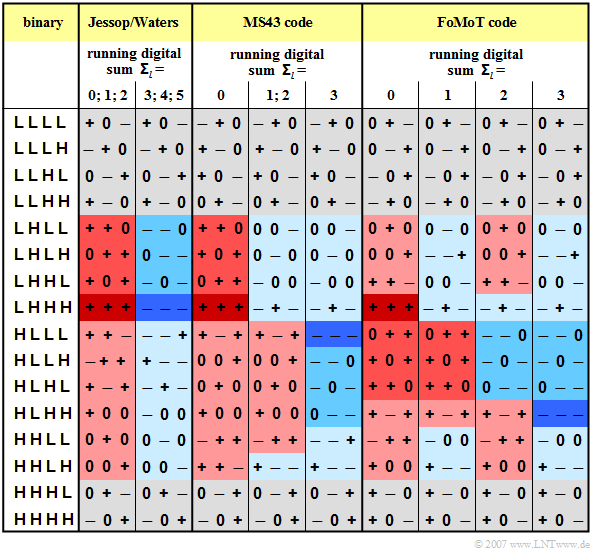
The table shows the coding rules for the three 4B3T codes mentioned above. To simplify the notation,
- "+" stands for the amplitude coefficient "+1" and
- "–" for the coefficient "–1".
You can seee from the graph:
- The two code tables of the Jessop–Waters code are selected in such a way that the running digital sum ${\it \Sigma}_l$ always lies between $0$ and $5$.
- For the other two codes (MS43, FoMoT), the restriction of the running digital sum to the range $0 \le {\it \Sigma}_l \le 3$ is achieved by three resp. four alternative tables.
ACF and PSD of the 4B3T codes
The procedure for calculating the auto-correlation function $\rm (ACF)$ and the power-spectral density $\rm (PSD)$ is only outlined here in bullet points:
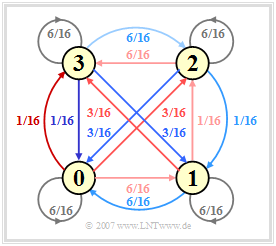
(1) The transition of the running digital sum from ${\it \Sigma}_l$ to ${\it \Sigma}_{l+1}$ is described by a homogeneous stationary first-order Markov chain with six $($Jessop–Waters$)$ or four states $($MS43, FoMoT$)$. For the FoMoT code, the Markov diagram sketched on the right applies.
(2) The values at the arrows denote the transition probabilities ${\rm Pr}({\it \Sigma}_{l+1}|{\it \Sigma}_{l})$, resulting from the respective code tables. The colors correspond to the backgrounds of the table on the last section. Due to the symmetry of the FoMoT Markov diagram, the four probabilities are all the same:
- $${\rm Pr}({\it \Sigma}_{l} = 0) = \text{...} = {\rm Pr}({\it \Sigma}_{l} = 3) = 1/4.$$
(3) The auto-correlation function $\varphi_a(\lambda) = {\rm E}\big [a_\nu \cdot a_{\nu+\lambda}\big ]$ of the amplitude coefficients can be determined from this diagram. Simpler than the analytical calculation, which requires a very large computational effort, is the simulative determination of the ACF values by computer.
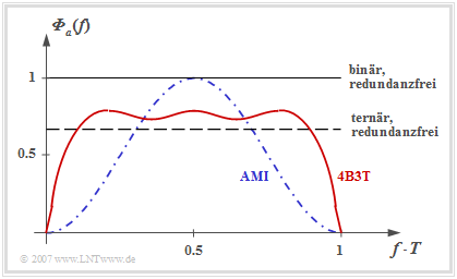
Fourier transforming the ACF yields the power-spectral density ${\it \Phi}_a(f)$ of the amplitude coefficients corresponding to the following graph from [TS87][1]. The outlined PSD was determined for the FoMoT code, whose Markov diagram is shown above. The differences between the individual 4B3T codes are not particularly pronounced. Thus, for the MS43 code ${\rm E}\big [a_\nu^2 \big ] \approx 0.65$ and for the other two 4B3T codes (Jessop/Waters, MS43) ${\rm E}\big [a_\nu^2 \big ] \approx 0.69$.
The statements of this graph can be summarized as follows:
- The graph shows the power-spectral density ${\it \Phi}_a(f)$ of the amplitude coefficients $a_\nu$ of the 4B3T code ⇒ red curve.
- The PSD ${\it \Phi}_s(f)$ including the basic transmission pulse is obtained by multiplying by $1/T \cdot |G_s(f)|^2$. For example, ${\it \Phi}_a(f)$ must be multiplied by a $\rm sinc^2$ function, if $g_s(t)$ describes a rectangular pulse.
- Redundancy-free binary or ternary coding results in a constant ${\it \Phi}_a(f)$ in each case, the magnitude of which depends on the number $M$ of levels (different signal power).
- In contrast, the 4B3T power-spectral density has zeros at $f = 0$ and multiples of $f = 1/T$.
- The zero point at $f = 0$ has the advantage that the 4B3T signal can also be transmitted without major losses via a so-called "telephone channel", which is not suitable for a DC signal due to transformers.
- The zero point at $f = 1/T$ has the disadvantage that this makes clock recovery at the receiver more difficult. Outside of these zeros, the 4B3T codes have a flatter ${\it \Phi}_a(f)$ than the AMI code discussed in the next chapter (blue curve), which is advantageous.
- The reason for the flatter PSD curve at medium frequencies as well as the steeper drop towards the zeros is that for the 4B3T codes up to five $+1$ coefficients (resp. $-1$ coefficients) can follow each other. With the AMI code, these symbols occur only in isolation.
Error probability of the 4B3T codes
We now consider the symbol error probability when using the 4B3T code in comparison with redundancy-free binary and ternary coding, subject to the following conditions:
- The system comparison is first made under the constraint of "peak limitation". Therefore, we use the rectangular basic transmission pulse, which is optimal for this purpose.
- The overall frequency response shows a cosine rolloff with best possible rolloff factor $r = 0.8$. The noise power $\sigma_d^2$ is thus $12\%$ larger than with the matched filter (global optimum), see graph in the section "Optimization of the rolloff factor with peak limitation" in the third main chapter.
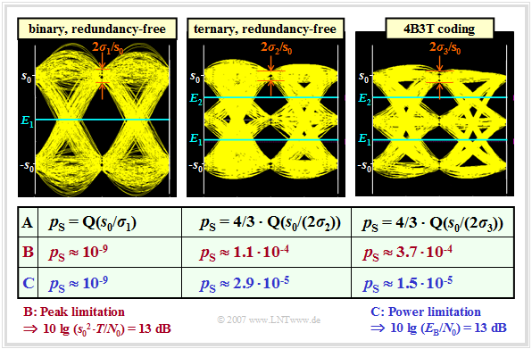
The following graph shows the eye diagrams (with noise) of the three systems to be compared. It also contains $($in row $\rm A)$ the equations for calculating the symbol error probability. Approximately 2000 eye lines are drawn for each diagram.
The first two rows of the table describe the system comparison at peak limitation. For the binary system (first column), the noise power (taking into account the $12\%$ increase) is given by
- $$\sigma_d^2 = 1.12 \cdot {N_0}/({2 \cdot T}) = 0.56 \cdot {N_0}/{T} = \sigma_1^2 \hspace{0.05cm}.$$
For the eye diagram and the following calculations, a signal-to-noise ratio of $10 \cdot \lg \hspace{0.05cm}(s_0^2 \cdot T/N_0) = 13 \ \rm dB$ is assumed in each case. This gives:
- $$10 \cdot {\rm lg } \hspace{0.1cm}{s_0^2 \cdot T}/{N_0} = 13 \, {\rm dB } \hspace{0.3cm} \Rightarrow \hspace{0.3cm}{s_0^2 \cdot T}/{N_0} = 10^{1.3} \approx 20 \hspace{0.3cm} \Rightarrow \hspace{0.3cm}\sigma_1^2 = 0.56 \cdot {s_0^2}/{20} \approx 0.028 \cdot s_0^2 \hspace{0.3cm} \Rightarrow \hspace{0.3cm}{ \sigma_1}/{s_0}\approx 0.167 \hspace{0.05cm}.$$
Row $\rm B$ shows the associated symbol error probability $p_{\rm S} \approx {\rm Q}(s_0/\sigma_1) \approx {\rm Q}(6) = 10^{-9}$.
The two other eye diagrams can be interpreted as follows:
- For the redundancy-free ternary system, the eye opening is only half as large as in the binary case, and the noise power $\sigma_2^2$ is smaller than $\sigma_1^2$ by a factor of $\log_2 \hspace{0.05cm}(3)$. The factor $4/3$ in front of the Q–function takes into account that the ternary "0" can be distorted in both directions. This results in the following numerical values:
- $$\frac{ \sigma_2}{s_0}\hspace{-0.05cm} =\hspace{-0.05cm} \frac{ \sigma_1/s_0}{\sqrt{{\rm log_2} (3)}}\hspace{-0.05cm} =\hspace{-0.05cm}\frac{ 0.167}{1.259} \approx 0.133 \hspace{0.3cm} \Rightarrow \hspace{0.3cm}p_{\rm S}\hspace{-0.05cm}=\hspace{-0.05cm} {4}/{3} \cdot {\rm Q}\left (\frac{ 0.5}{0.133}\right)\approx {4}/{3} \cdot {\rm Q}(3.76) \hspace{-0.05cm}= \hspace{-0.05cm}1.1 \cdot 10^{-4} .$$
- The 4B3T code yields even slightly less favorable results, since here the noise power $(\sigma_3^2)$ is reduced less than in the redundancy-free ternary code $(\sigma_2^2)$ for the same eye opening:
- $$\frac{ \sigma_3}{s_0} = \frac{ \sigma_1/s_0}{\sqrt{4/3}} =\frac{ 0.167}{1.155} \approx 0.145 \hspace{0.3cm} \Rightarrow \hspace{0.3cm}p_{\rm S}= {4}/{3} \cdot {\rm Q}\left (\frac{ 0.5}{0.145}\right)\approx {4}/{3} \cdot {\rm Q}(3.45) = 3.7 \cdot 10^{-4} \hspace{0.05cm}.$$
$\text{Row C: Symbol error probabilities under power limitation}$
For the following is given: $10 \cdot \lg \hspace{0.05cm}(E_{\rm B}/N_0) = 13 \ \rm dB$:
- For the redundancy-free binary system with NRZ rectangular pulses, $p_{\rm S}$ is not changed with respect to row $\rm B$ because of $E_{\rm B} = s_0^2 \cdot T$:
- $$p_\text{S, power limitation} = p_\text{S, peak limitation} \approx 10^{-9}.$$
- For the two ternary codes, ${\rm E}\big [a_\nu^2\big ] \approx 2/3$. Therefore, the amplitude can here be increased by a factor of $\sqrt{(3/2)} \approx 1.225$.
- For the redundancy-free ternary code, one thus obtains with power limitation an error probability smaller by factor $ 4$ than with peak limitation $($cf. rows $\rm B$ and $\rm C)$:
- $$p_\text{S, power limitation} = 4/3 \cdot {\rm Q}(1.225 \cdot 3.76) \approx 2.9 \cdot 10^{-5} \approx 0.26 \cdot p_\text{S, peak limitation} .$$
- A similar (and even stronger) result holds for the 4B3T code:
- $$p_\text{S, power limitation} = 4/3 \cdot {\rm Q}(1.225 \cdot 3.45) \approx 1.5 \cdot 10^{-5} \approx 0.04 \cdot p_\text{S, peak limitation}.$$
Exercises for the chapter
Exercise 2.6: Modified MS43 Code
Exercise 2.6Z: 4B3T Code according to Jessop and Waters
References
- ↑ Tröndle, K.; Söder, G.: Optimization of Digital Transmission Systems. Boston – London: Artech House, 1987, ISBN: 0-89006-225-0.


