Channel Coding/Decoding of Convolutional Codes

1. Channel Coding
2. Convolutional Codes and Their Decoding
3. Decoding of Convolutional Codes

• Previous page
• Next page

• Previous page
• Next page

Block diagram and requirements

A significant advantage of convolutional coding is that there is a very efficient decoding method for this in the form of the  "Viterbi algorithm".  This algorithm,  developed by  $\text{Andrew James Viterbi}$  has already been described in the chapter  "Viterbi receiver"  of the book "Digital Signal Transmission" with regard to its use for equalization.

For its use as a convolutional decoder we assume the block diagram on the right and the following prerequisites:

System model for the decoding of convolutional codes

• The information sequence  $\underline{u} = (u_1, \ u_2, \ \text{... } \ )$  is here in contrast to the description of linear block codes   ⇒   "first main chapter"  or of Reed–Solomon codes   ⇒   "second main chapter"  generally infinitely long  ("semi–infinite").  For the information symbols always applies  $u_i ∈ \{0, 1\}$.
  

• The encoded sequence  $\underline{x} = (x_1, \ x_2, \ \text{... })$  with  $x_i ∈ \{0, 1\}$  depends not only on   $\underline{u}$   but also on the code rate  $R = 1/n$, the memory  $m$  and the transfer function matrix  $\mathbf{G}(D)$  . For finite number  $L$  of information bits,  the convolutional code should be terminated by appending  $m$  zeros:

\[\underline{u}= (u_1,\hspace{0.05cm} u_2,\hspace{0.05cm} \text{...} \hspace{0.1cm}, u_L, \hspace{0.05cm} 0 \hspace{0.05cm},\hspace{0.05cm} \text{...} \hspace{0.1cm}, 0 ) \hspace{0.3cm}\Rightarrow \hspace{0.3cm} \underline{x}= (x_1,\hspace{0.05cm} x_2,\hspace{0.05cm} \text{...} \hspace{0.1cm}, x_{2L}, \hspace{0.05cm} x_{2L+1} ,\hspace{0.05cm} \text{...} \hspace{0.1cm}, \hspace{0.05cm} x_{2L+2m} ) \hspace{0.05cm}.\]

• The received sequence  $\underline{y} = (y_1, \ y_2, \ \text{...} )$  results according to the assumed channel model. For a digital model like the  $\text{Binary Symmetric Channel}$  $\rm (BSC)$  holds   $y_i ∈ \{0, 1\}$,  so the falsification from  $\underline{x}$  to  $\underline{y}$   can be quantified with the  $\text{Hamming distance}$  $d_{\rm H}(\underline{x}, \underline{y})$.

• The required modifications for the  $\text{AWGN channel}$  follow in the section  "Viterbi algorithm based on correlation and metrics".

• The Viterbi algorithm provides an estimate  $\underline{z}$  for the encoded sequence  $\underline{x}$  and another estimate  $\underline{v}$  for the information sequence  $\underline{u}$.  Thereby holds:

\[{\rm Pr}(\underline{z} \ne \underline{x})\stackrel{!}{=}{\rm Minimum} \hspace{0.25cm}\Rightarrow \hspace{0.25cm} {\rm Pr}(\underline{\upsilon} \ne \underline{u})\stackrel{!}{=}{\rm Minimum} \hspace{0.05cm}.\]

$\text{Conclusion:}$  Given a digital channel model   $($for example,   the BSC model$)$,   the Viterbi algorithm searches from all possible encoded sequences  $\underline{x}\hspace{0.05cm}'$  the sequence  $\underline{z}$  with the minimum Hamming distance   $d_{\rm H}(\underline{x}\hspace{0.05cm}', \underline{y})$   to the received sequence  $\underline{y}$:

\[\underline{z} = {\rm arg} \min_{\underline{x}\hspace{0.05cm}' \in \hspace{0.05cm} \mathcal{C} } \hspace{0.1cm} d_{\rm H}( \underline{x}\hspace{0.05cm}'\hspace{0.02cm},\hspace{0.02cm} \underline{y} ) = {\rm arg} \max_{\underline{x}' \in \hspace{0.05cm} \mathcal{C} } \hspace{0.1cm} {\rm Pr}( \underline{y} \hspace{0.05cm} \vert \hspace{0.05cm} \underline{x}')\hspace{0.05cm}.\]

• This also means:   The Viterbi algorithm satisfies the  $\text{maximum likelihood criterion}$.

Preliminary remarks on the following decoding examples

Trellis for decoding the received sequence  $\underline{y}$

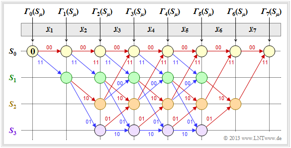
The following  »prerequisites«   apply to all examples in this chapter:

• Standard convolutional encoder:   Rate $R = 1/2$,  memory  $m = 2$;

• transfer function matrix:   $\mathbf{G}(D) = (1 + D + D^2, 1 + D^2)$;

• length of information sequence:   $L = 5$;

• consideration of termination:   $L\hspace{0.05cm}' = 7$;

• length of sequences  $\underline{x}$  and  $\underline{y}$ :   $14$  bits each;

• allocation according to  $\underline{y} = (\underline{y}_1, \ \underline{y}_2, \ \text{...} \ , \ \underline{y}_7)$
  ⇒   bit pairs  $\underline{y}_i ∈ \{00, 01, 10, 11\}$;
• Viterbi decoding using trellis diagram:

red arrow   ⇒   hypothesis  $u_i = 0$,

blue arrow   ⇒   hypothesis  $u_i = 1$;

• hypothetical code sequence  $\underline{x}_i\hspace{0.01cm}' ∈ \{00, 01, 10, 11\}$;

• all hypothetical quantities with apostrophe.

We always assume that the Viterbi decoding is based at the  $\text{Hamming distance}$  $d_{\rm H}(\underline{x}_i\hspace{0.01cm}', \ \underline{y}_i)$  between the received word  $\underline{y}_i$  and the four possible code words  $x_i\hspace{0.01cm}' ∈ \{00, 01, 10, 11\}$.  We then proceed as follows:

• In the still empty circles the error value  ${\it \Gamma}_i(S_{\mu})$  of states  $S_{\mu} (0 ≤ \mu ≤ 3)$  at time points  $i$  are entered.  The initial value is always  ${\it \Gamma}_0(S_0) = 0$.

• The error values for  $i = 1$  and  $i = 2$  are given by

\[{\it \Gamma}_1(S_0) =d_{\rm H} \big ((00)\hspace{0.05cm},\hspace{0.05cm} \underline{y}_1 \big ) \hspace{0.05cm}, \hspace{2.38cm}{\it \Gamma}_1(S_1) = d_{\rm H} \big ((11)\hspace{0.05cm},\hspace{0.05cm} \underline{y}_1 \big ) \hspace{0.05cm},\]

\[{\it \Gamma}_2(S_0) ={\it \Gamma}_1(S_0) + d_{\rm H} \big ((00)\hspace{0.05cm},\hspace{0.05cm} \underline{y}_2 \big )\hspace{0.05cm}, \hspace{0.6cm}{\it \Gamma}_2(S_1) = {\it \Gamma}_1(S_0)+ d_{\rm H} \big ((11)\hspace{0.05cm},\hspace{0.05cm} \underline{y}_2 \big ) \hspace{0.05cm},\hspace{0.6cm}{\it \Gamma}_2(S_2) ={\it \Gamma}_1(S_1) + d_{\rm H} \big ((10)\hspace{0.05cm},\hspace{0.05cm} \underline{y}_2 \big )\hspace{0.05cm}, \hspace{0.6cm}{\it \Gamma}_2(S_3) = {\it \Gamma}_1(S_1)+ d_{\rm H} \big ((01)\hspace{0.05cm},\hspace{0.05cm} \underline{y}_2 \big ) \hspace{0.05cm}.\]

• From  $i = 3$  the trellis has reached its basic form, and to compute all  ${\it \Gamma}_i(S_{\mu})$  the minimum between two sums must be determined in each case:

\[{\it \Gamma}_i(S_0) ={\rm Min} \left [{\it \Gamma}_{i-1}(S_0) + d_{\rm H} \big ((00)\hspace{0.05cm},\hspace{0.05cm} \underline{y}_i \big )\hspace{0.05cm}, \hspace{0.2cm}{\it \Gamma}_{i-1}(S_2) + d_{\rm H} \big ((11)\hspace{0.05cm},\hspace{0.05cm} \underline{y}_i \big ) \right ] \hspace{0.05cm},\]

\[{\it \Gamma}_i(S_1)={\rm Min} \left [{\it \Gamma}_{i-1}(S_0) + d_{\rm H} \big ((11)\hspace{0.05cm},\hspace{0.05cm} \underline{y}_i \big )\hspace{0.05cm}, \hspace{0.2cm}{\it \Gamma}_{i-1}(S_2) + d_{\rm H} \big ((00)\hspace{0.05cm},\hspace{0.05cm} \underline{y}_i \big ) \right ] \hspace{0.05cm},\]

\[{\it \Gamma}_i(S_2) ={\rm Min} \left [{\it \Gamma}_{i-1}(S_1) + d_{\rm H} \big ((10)\hspace{0.05cm},\hspace{0.05cm} \underline{y}_i \big )\hspace{0.05cm}, \hspace{0.2cm}{\it \Gamma}_{i-1}(S_3) + d_{\rm H} \big ((01)\hspace{0.05cm},\hspace{0.05cm} \underline{y}_i \big ) \right ] \hspace{0.05cm},\]

\[{\it \Gamma}_i(S_3) ={\rm Min} \left [{\it \Gamma}_{i-1}(S_1) + d_{\rm H} \big ((01)\hspace{0.05cm},\hspace{0.05cm} \underline{y}_i \big )\hspace{0.05cm}, \hspace{0.2cm}{\it \Gamma}_{i-1}(S_3) + d_{\rm H} \big ((10)\hspace{0.05cm},\hspace{0.05cm} \underline{y}_i \big ) \right ] \hspace{0.05cm}.\]

• Of the two branches arriving at a node  ${\it \Gamma}_i(S_{\mu})$  the worse one  $($which would have led to a larger  ${\it \Gamma}_i(S_{\mu})$  is eliminated.  Only one branch then leads to each node.
  

• Once all error values up to and including  $i = 7$  have been determined,  the Viterbi algotithm can be completed by searching the  "connected path"  from the end of the trellis   ⇒   ${\it \Gamma}_7(S_0)$  to the beginning   ⇒   ${\it \Gamma}_0(S_0)$ .

• Through this path,  the most likely code sequence  $\underline{z}$  and the most likely information sequence  $\underline{v}$  are then fixed.

• Not all received sequences are transmitted error-free  $(\underline{y} =\underline{x})$,  however often holds with Viterbis decoding:   $\underline{z} = \underline{x}$  and  $\underline{v} = \underline{u}$.

• But if there are too many transmission errors,  the Viterbi algorithm also fails.
  

Creating the trellis in the error-free case  –  Acumulated error value calculation

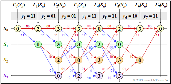
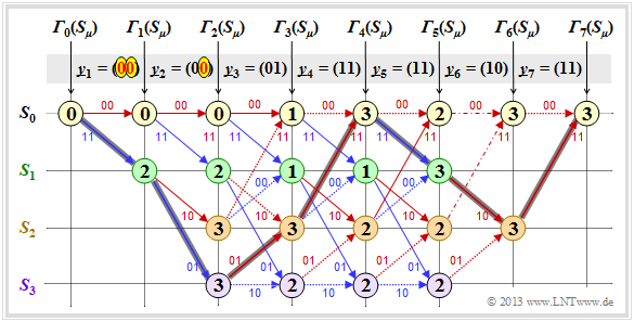
First,  we assume the received sequence  $\underline{y} = (11, 01, 01, 11, 11, 10, 11)$  which is here already subdivided into bit pairs: 

$$\underline{y}_1, \hspace{0.05cm} \text{...} \hspace{0.05cm} , \ \underline{y}_7.$$

The numerical values entered in the trellis and the different types of strokes are explained in the following text.

Viterbi scheme for the received vector  $\underline{y} = (11, 01, 01, 11, 11, 10, 11)$

• Starting from the initial value  ${\it \Gamma}_0(S_0) = 0$  we get  $\underline{y}_1 = (11)$  by adding the Hamming distances

$$d_{\rm H}((00), \ \underline{y}_1) = 2\hspace{0.6cm} \text{or} \hspace{0.6cm}d_{\rm H}((11), \ \underline{y}_1) = 0$$

to the  "$($acumulated$)$ error values"   ${\it \Gamma}_1(S_0) = 2, \ {\it \Gamma}_1(S_1) = 0$.

• In the second decoding step there are error values for all four states:   With  $\underline{y}_2 = (01)$  one obtains:

\[{\it \Gamma}_2(S_0) = {\it \Gamma}_1(S_0) + d_{\rm H} \big ((00)\hspace{0.05cm},\hspace{0.05cm} (01) \big ) = 2+1 = 3 \hspace{0.05cm},\]

\[{\it \Gamma}_2(S_1) ={\it \Gamma}_1(S_0) + d_{\rm H} \big ((11)\hspace{0.05cm},\hspace{0.05cm} (01) \big ) = 2+1 = 3 \hspace{0.05cm},\]

\[{\it \Gamma}_2(S_2) ={\it \Gamma}_1(S_1) + d_{\rm H} \big ((10)\hspace{0.05cm},\hspace{0.05cm} (01) \big ) = 0+2=2 \hspace{0.05cm},\]

\[{\it \Gamma}_2(S_3) = {\it \Gamma}_1(S_1) + d_{\rm H} \big ((01)\hspace{0.05cm},\hspace{0.05cm} (01) \big ) = 0+0=0 \hspace{0.05cm}.\]

• In all further decoding steps,  two values must be compared in each case,  whereby the node  ${\it \Gamma}_i(S_{\mu})$  is always assigned the smaller value.

• For example,  for  $i = 3$  with  $\underline{y}_3 = (01)$:

\[{\it \Gamma}_3(S_0) ={\rm min} \left [{\it \Gamma}_{2}(S_0) + d_{\rm H} \big ((00)\hspace{0.05cm},\hspace{0.05cm} (01) \big )\hspace{0.05cm}, \hspace{0.2cm}{\it \Gamma}_{2}(S_2) + d_{\rm H} \big ((11)\hspace{0.05cm},\hspace{0.05cm} (01) \big ) \right ] ={\rm min} \big [ 3+1\hspace{0.05cm},\hspace{0.05cm} 2+1 \big ] = 3\hspace{0.05cm},\]

\[{\it \Gamma}_3(S_3) ={\rm min} \left [{\it \Gamma}_{2}(S_1) + d_{\rm H} \big ((01)\hspace{0.05cm},\hspace{0.05cm} (01) \big )\hspace{0.05cm}, \hspace{0.2cm}{\it \Gamma}_{2}(S_3) + d_{\rm H} \big ((10)\hspace{0.05cm},\hspace{0.05cm} (01) \big ) \right ] ={\rm min} \big [ 3+0\hspace{0.05cm},\hspace{0.05cm} 0+2 \big ] = 2\hspace{0.05cm}.\]

• In the considered example,  from  $i = 6$  the termination of the convolutional code becomes effective.  Here,  only two comparisons are left to determine  ${\it \Gamma}_6(S_0) = 3$  and  ${\it \Gamma}_6(S_2)= 0$  and for  $i = 7$  only one comparison with the final rror value  ${\it \Gamma}_7(S_0) = 0$.
  

The description of the Viterbi decoding process continues in the next section.

Evaluating the trellis in the error-free case  –  Path search

After all error values  ${\it \Gamma}_i(S_{\mu})$  have been determined  $($ in the present example for  $1 ≤ i ≤ 7$  and  $0 ≤ \mu ≤ 3)$,  the Viterbi decoder can start the path search:

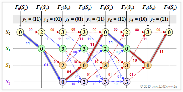
1.   The following graph shows the trellis after the error value calculation.  All circles are assigned numerical values.
2.   However,  the most probable path already drawn in the graphic is not yet known.
3.   In the following,  of course,  no use is made of the  "error-free case"  information already contained in the heading.
4.   Of the two branches arriving at a node,  only the one that led to the minimum error value  ${\it \Gamma}_i(S_{\mu})$  is used for the final path search.
5.   The  "bad"  branches are discarded.  They are each shown dotted in the above graph.

Viterbi path search for for the received vector  $\underline{y} = (11, 01, 01, 11, 11, 10, 11)$

The path search runs as follows:

• Starting from the end value  ${\it \Gamma}_7(S_0)$  a continuous path is searched in backward direction to the start value  ${\it \Gamma}_0(S_0)$.  Only the solid branches are allowed.  Dotted lines cannot be part of the selected  $($best$)$  path.
  

• The selected path  $($grayed out in the graph$)$  traverses from right to left in the sketch the states is 

$$S_0 ← S_2 ← S_1 ← S_0 ← S_2 ← S_3 ← S_1 ← S_0.$$

There is no second continuous path from  ${\it \Gamma}_7(S_0)$  to  ${\it \Gamma}_0(S_0)$. This means:   The decoding result is unique.

• The result  $\underline{v} = (1, 1, 0, 0, 1, 0, 0)$  of the Viterbi decoder with respect to the information sequence is obtained if for the continuous path  $($but now in forward direction from left to right$)$  the colors of the individual branches are evaluated  $($red   ⇒   "$0$",   blue   ⇒   $1)$.
  
  

From the final value   ${\it \Gamma}_7(S_0) = 0$   it can be seen that there were no transmission errors in this first example:

• The decoding result  $\underline{z}$  thus matches the received vector  $\underline{y} = (11, 01, 01, 11, 11, 10, 11)$  and the actual encoded sequence  $\underline{x}$.

• With error-free transmission,  $ \underline{v}$  is not only the most probable info sequence  $\underline{u}$  according to the maximum likelihood criterion,  but both are even identical:   $\underline{v} \equiv \underline{u}$.
  

Decoding examples for the erroneous case

Now follow three examples of Viterbi decoding for the errorneous case.

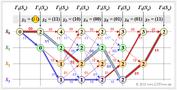
$\text{Example 1:}$  We assume here the received vector  $\underline{y} = \big (11\hspace{0.05cm}, 11\hspace{0.05cm}, 10\hspace{0.05cm}, 00\hspace{0.05cm}, 01\hspace{0.05cm}, 01\hspace{0.05cm}, 11 \hspace{0.05cm} \hspace{0.05cm} \big ) $  which does not represent a valid code sequence  $\underline{x}$ . The calculation of error values  ${\it \Gamma}_i(S_{\mu})$  and the path search is done as described in section  "Preliminaries"  and demonstrated in the last two sections for the error-free case.

Decoding example with two bit errors at the beginning

As summary of this first example,  it should be noted:

• Also with tis trellis,  a unique path  $($with dark gray background$)$  can be traced,  leading to the following results  $($recognizable by the labels or the colors of this path$)$:

\[\underline{z} = \big (00\hspace{0.05cm}, 11\hspace{0.05cm}, 10\hspace{0.05cm}, 00\hspace{0.05cm}, 01\hspace{0.05cm}, 01\hspace{0.05cm}, 11 \hspace{0.05cm} \big ) \hspace{0.05cm},\]

\[ \underline{\upsilon} =\big (0\hspace{0.05cm}, 1\hspace{0.05cm}, 0\hspace{0.05cm}, 1\hspace{0.05cm}, 1\hspace{0.05cm}, 0\hspace{0.05cm}, 0 \hspace{0.05cm} \big ) \hspace{0.05cm}.\]

• Comparing the most likely transmitted code sequence  $\underline{z}$  with the received vector  $\underline{y}$  shows that there were two bit errors directly at the beginning.  But since the used convolutional code has the $\text{free distance}$  $d_{\rm F} = 5$,  two transmission errors do not yet lead to a wrong decoding result.
  

• There are other paths such as the lighter highlighted path

$$S_0 → S_1 → S_3 → S_3 → S_3 → S_2 → S_0 → S_0$$

that initially appear to be promising.  Only in the last decoding step  $(i = 7)$  can this light gray path finally be discarded.

Further remarks:

1. The example shows that a too early decision is often not purposeful. 
2. One can also see the expediency of termination:   With final decision at  $i = 5$  $($end of information sequence$)$,  the sequences  $(0, 1, 0, 1, 1)$  and  $(1, 1, 1, 1, 0)$  would still have been considered equally likely.
3. In the calculation of  ${\it \Gamma}_5(S_0) = 3$  and  ${\it \Gamma}_5(S_1) = 3$  here in each case the two comparison branches lead to exactly the same minimum error value. In the graph these two special cases are marked by dash dots.  In this example,  this special case has no effect on the path search.
4. Nevertheless,  the algorithm always expects a decision between two competing branches.  In practice,  one helps by randomly selecting one of the two paths if they are equal.

$\text{Example 2:}$  In this example,  we assume the following assumptions regarding source and encoder:

Decoding example with three bit errors

$$\underline{u} = \big (1\hspace{0.05cm}, 1\hspace{0.05cm}, 0\hspace{0.05cm}, 0\hspace{0.05cm}, 1 \hspace{0.05cm}, 0\hspace{0.05cm}, 0 \big )$$

$$\Rightarrow \hspace{0.3cm} \underline{x} = \big (11\hspace{0.05cm}, 01\hspace{0.05cm}, 01\hspace{0.05cm}, 11\hspace{0.05cm}, 11\hspace{0.05cm}, 10\hspace{0.05cm}, 11 \hspace{0.05cm} \hspace{0.05cm} \big ) \hspace{0.05cm}.$$

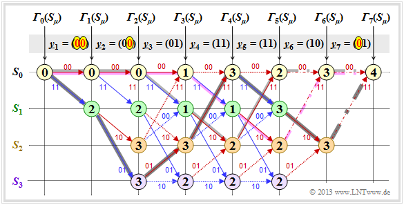
From the graph you can see here that the decoder decides for the correct path  $($dark background$)$  despite three bit errors.

• So there is not always a wrong decision,nbsp; if more than  $d_{\rm F}/2$  bit errors occurred.

• But with statistical distribution of the three bit errors,nbsp; wrong decision would be more frequent than right.

$\text{Example 3:}$  Here also applies 

Decoding example with four bit errors

$$\underline{u} = \big (1\hspace{0.05cm}, 1\hspace{0.05cm}, 0\hspace{0.05cm}, 0\hspace{0.05cm}, 1 \hspace{0.05cm}, 0\hspace{0.05cm}, 0 \big )$$

$$\Rightarrow \hspace{0.3cm} \underline{x} = \big (11\hspace{0.05cm}, 01\hspace{0.05cm}, 01\hspace{0.05cm}, 11\hspace{0.05cm}, 11\hspace{0.05cm}, 10\hspace{0.05cm}, 11 \hspace{0.05cm} \hspace{0.05cm} \big ) \hspace{0.05cm}.$$

Unlike the last example,  a fourth bit error is added:  $\underline{y}_7 = (01).$

• Now both branches in step  $i = 7$  lead to the minimum error value  ${\it \Gamma}_7(S_0) = 4$,  recognizable by the dash-dotted transitions.

• If one decides in the then required lottery procedure for the path with dark background,  the correct decision is still made even with four bit errors:   $\underline{v} = \big (1\hspace{0.05cm}, 1\hspace{0.05cm}, 0\hspace{0.05cm}, 0\hspace{0.05cm}, 1 \hspace{0.05cm}, 0\hspace{0.05cm}, 0 \big )$.
  

• Otherwise,  a wrong decision is made. Depending on the outcome of the dice roll in step  $i =6$  between the two dash-dotted competitors,  you choose either the purple or the light gray path. 

• Both have little in common with the correct path.

Relationship between Hamming distance and correlation

Especially for the  $\text{BSC model}$  $($but also for any other binary channel  ⇒   input  $x_i ∈ \{0,1\}$,  output $y_i ∈ \{0,1\}$  such as the  $\text{Gilbert–Elliott model}$$)$  provides

• the Hamming distance  $d_{\rm H}(\underline{x}, \ \underline{y})$  exactly the same information about the similarity of the input sequence  $\underline{x}$  and the output sequence  $\underline{y}$ 

• as the  $\text{inner product}$.  Assuming that the sequences are in bipolar form  $($denoted by tildes$)$  and that the sequence length is  $L$  in each case,  the inner product is:

\[<\hspace{-0.1cm}\underline{\tilde{x}}, \hspace{0.05cm}\underline{\tilde{y}} \hspace{-0.1cm}> \hspace{0.15cm} = \sum_{i = 1}^{L} \tilde{x}_i \cdot \tilde{y}_i \hspace{0.3cm}{\rm with } \hspace{0.2cm} \tilde{x}_i = 1 - 2 \cdot x_i \hspace{0.05cm},\hspace{0.2cm} \tilde{y}_i = 1 - 2 \cdot y_i \hspace{0.05cm},\hspace{0.2cm} \tilde{x}_i, \hspace{0.05cm}\tilde{y}_i \in \hspace{0.1cm}\{ -1, +1\} \hspace{0.05cm}.\]

We sometimes refer to this inner product as the  »correlation value«.  Unlike the   $\text{correlation coefficient}$  the  "correlation value"  may well exceed the range of values  $±1$.

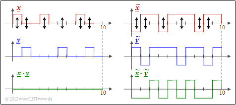
$\text{Example 4:}$  We consider here two binary sequences of length  $L = 10$.  Shown on the left are the  »unipolar«  sequences  $\underline{x}$  and  $\underline{y}$  and the product  $\underline{x} \cdot \underline{y}$.

Relationship between Haming distance and correlation value

• You can see the Hamming distance  $d_{\rm H}(\underline{x}, \ \underline{y}) = 6$   ⇒   six bit errors at the arrow positions.

• The inner product   $ < \underline{x} \cdot \underline{y} > \hspace{0.15cm} = \hspace{0.15cm}0$   has no significance here.  For example,  $< \underline{0} \cdot \underline{y} > $ is always zero regardless of  $\underline{y}$.

The Hamming distance  $d_{\rm H} = 6$  can also be seen from the  »bipolar«  $($antipodal$)$ plot in the right graph.

• The  "correlation value"  has now the correct value:

$$4 \cdot (+1) + 6 \cdot (-1) = \, -2.$$

• For the deterministic relationship between the  "correlation value"  and the  "Hamming distance"  holds with the sequence length  $L$:

$$ < \underline{ \tilde{x} } \cdot \underline{\tilde{y} } > \hspace{0.15cm} = \hspace{0.15cm} L - 2 \cdot d_{\rm H} (\underline{\tilde{x} }, \hspace{0.05cm}\underline{\tilde{y} })\hspace{0.05cm}. $$

$\text{Conclusion:}$  Let us now interpret this last equation for some special cases:

• »Identical sequences«:   The Hamming distance is equal  $0$  and the  correlation value is equal  $L$.
  

• »Inverted sequences«:   The Hamming distance is equal to  $L$  and the  correlation value  is equal to  $-L$.
  

• »Uncorrelated sequences«:   The Hamming distance is equal to  $L/2$  and the  correlation value  is equal to  $0$.

Viterbi algorithm based on correlation and metrics

Using the insights of the last section,  the Viterbi algorithm can also be characterized as follows.

$\text{Alternative description:}$ 

• The Viterbi algorithm searches from all possible code sequences  $\underline{x}' ∈ \mathcal{C}$  the sequence  $\underline{z}$  with the  »maximum correlation value«  to the received sequence  $\underline{y}$:

\[\underline{z} = {\rm arg} \max_{\underline{x}' \in \hspace{0.05cm} \mathcal{C} } \hspace{0.1cm} \left\langle \tilde{\underline{x} }'\hspace{0.05cm} ,\hspace{0.05cm} \tilde{\underline{y} } \right\rangle \hspace{0.4cm}{\rm with }\hspace{0.4cm}\tilde{\underline{x} }\hspace{0.05cm}'= 1 - 2 \cdot \underline{x}'\hspace{0.05cm}, \hspace{0.2cm} \tilde{\underline{y} }= 1 - 2 \cdot \underline{y} \hspace{0.05cm}.\]

• Here,  $〈\ \text{ ...} \ 〉$  denotes a  "correlation value"  according to the statements in the last section.  The tildes again indicate the bipolar representation.

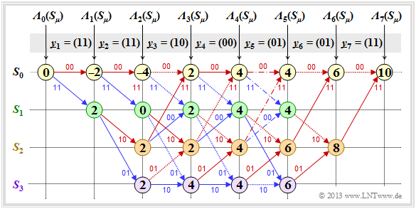
The graphic shows the corresponding trellis evaluation. 

• As for the  $\text{Trellis evaluation according to Example 1}$  based on the minimum Hamming distance and the error values  ${\it \Gamma}_i(S_{\mu})$

• the the input sequence and the encoded sequence are

$$\underline{u} = \big (0\hspace{0.05cm}, 1\hspace{0.05cm}, 0\hspace{0.05cm}, 1\hspace{0.05cm}, 1\hspace{0.05cm}, 0\hspace{0.05cm}, 0 \hspace{0.05cm} \big ) \hspace{0.3cm} ⇒ \hspace{0.3cm} \underline{x} = \big (00, 11, 10, 00, 01, 01, 11 \big ) \hspace{0.05cm}.$$

Viterbi decoding based on correlation and metrics

Further are assumed:

• Standard convolutional encoder:   rate  $R = 1/2$,  memory  $m = 2$;

• the transfer function matrix:   $\mathbf{G}(D) = (1 + D + D^2, 1 + D^2)$;

• length of the information sequence:   $L = 5$;

• consideration of termination:  $L' = 7$;

• received vector   $\underline{y} = (11, 11, 10, 00, 01, 01, 11)$   ⇒   two bit errors;

• Viterbi decoding using trellis diagram:

• red arrow ⇒   hypothesis $u_i = 0$,
• blue arrow ⇒   hypothesis $u_i = 1$.

Adjacent trellis and the  $\text{Example 1 trellis}$   are very similar.  Just like the search for the sequence with the  "minimum Hamming distance",  the  "search for the maximum correlation value"  is also done step by step:

1.   The nodes here are called the  "cumulative metrics"  ${\it \Lambda}_i(S_{\mu})$.
2.   The  "branch metrics"  specify the  "metric increments".
   
3.   The final value  ${\it \Lambda}_7(S_0) = 10$  indicates the  "end correlation value"  between the selected sequence  $\underline{z}$  and the received vector  $\underline{y}$.
4.   In the error-free case,  the result would be  ${\it \Lambda}_7(S_0) = 14$.
   
   

$\text{Example 5:}$  The following detailed description of the trellis evaluation refer to the above trellis:

• The acumulated metrics at time  $i = 1$  result with  $\underline{y}_1 = (11)$  to

\[{\it \Lambda}_1(S_0) \hspace{0.15cm} = \hspace{0.15cm} <\hspace{-0.05cm}(00)\hspace{0.05cm}, \hspace{0.05cm}(11) \hspace{-0.05cm}>\hspace{0.2cm} = \hspace{0.2cm}<(+1,\hspace{0.05cm} +1)\hspace{0.05cm}, \hspace{0.05cm}(-1,\hspace{0.05cm} -1) >\hspace{0.1cm} = \hspace{0.1cm} -2 \hspace{0.05cm},\]

\[{\it \Lambda}_1(S_1) \hspace{0.15cm} = \hspace{0.15cm} <\hspace{-0.05cm}(11)\hspace{0.05cm}, \hspace{0.05cm}(11) \hspace{-0.05cm}>\hspace{0.2cm} = \hspace{0.2cm}<(-1,\hspace{0.05cm} -1)\hspace{0.05cm}, \hspace{0.05cm}(-1,\hspace{0.05cm} -1) >\hspace{0.1cm} = \hspace{0.1cm} +2 \hspace{0.05cm}.\]

• Accordingly,  at time  $i = 2$  with  $\underline{y}_2 = (11)$:

\[{\it \Lambda}_2(S_0) = {\it \Lambda}_1(S_0) \hspace{0.2cm}+ \hspace{0.1cm}<\hspace{-0.05cm}(00)\hspace{0.05cm}, \hspace{0.05cm}(11) \hspace{-0.05cm}>\hspace{0.2cm} = \hspace{0.1cm} -2-2 = -4 \hspace{0.05cm},\]

\[{\it \Lambda}_2(S_1) = {\it \Lambda}_1(S_0) \hspace{0.2cm}+ \hspace{0.1cm}<\hspace{-0.05cm}(11)\hspace{0.05cm}, \hspace{0.05cm}(11) \hspace{-0.05cm}>\hspace{0.2cm} = \hspace{0.1cm} -2+2 = 0 \hspace{0.05cm},\]

\[{\it \Lambda}_2(S_2)= {\it \Lambda}_1(S_1) \hspace{0.2cm}+ \hspace{0.1cm}<\hspace{-0.05cm}(10)\hspace{0.05cm}, \hspace{0.05cm}(11) \hspace{-0.05cm}>\hspace{0.2cm} = \hspace{0.1cm} +2+0 = +2 \hspace{0.05cm},\]

\[{\it \Lambda}_2(S_3)= {\it \Lambda}_1(S_1) \hspace{0.2cm}+ \hspace{0.1cm}<\hspace{-0.05cm}(01)\hspace{0.05cm}, \hspace{0.05cm}(11) \hspace{-0.05cm}>\hspace{0.2cm} = \hspace{0.1cm} +2+0 = +2 \hspace{0.05cm}.\]

• From time  $i =3$  a decision must be made between two acumulated metrics.  For example,  $\underline{y}_3 = (10)$  is obtained for the top and bottom metrics in the trellis:

\[{\it \Lambda}_3(S_0)={\rm max} \left [{\it \Lambda}_{2}(S_0) \hspace{0.2cm}+ \hspace{0.1cm}<\hspace{-0.05cm}(00)\hspace{0.05cm}, \hspace{0.05cm}(11) \hspace{-0.05cm}>\hspace{0.2cm} \hspace{0.05cm}, \hspace{0.2cm}{\it \Lambda}_{2}(S_1) \hspace{0.2cm}+ \hspace{0.1cm}<\hspace{-0.05cm}(00)\hspace{0.05cm}, \hspace{0.05cm}(11) \hspace{-0.05cm}> \right ] = {\rm max} \left [ -4+0\hspace{0.05cm},\hspace{0.05cm} +2+0 \right ] = +2\hspace{0.05cm},\]

\[{\it \Lambda}_3(S_3) ={\rm max} \left [{\it \Lambda}_{2}(S_1) \hspace{0.2cm}+ \hspace{0.1cm}<\hspace{-0.05cm}(01)\hspace{0.05cm}, \hspace{0.05cm}(10) \hspace{-0.05cm}>\hspace{0.2cm} \hspace{0.05cm}, \hspace{0.2cm}{\it \Lambda}_{2}(S_3) \hspace{0.2cm}+ \hspace{0.1cm}<\hspace{-0.05cm}(10)\hspace{0.05cm}, \hspace{0.05cm}(10) \hspace{-0.05cm}> \right ] = {\rm max} \left [ 0+0\hspace{0.05cm},\hspace{0.05cm} +2+2 \right ] = +4\hspace{0.05cm}.\]

• Comparing the  »accumulated correlation values«  ${\it \Lambda}_i(S_{\mu})$  to be maximized with the   »accumulated error values«  ${\it \Gamma}_i(S_{\mu})$  to be minimized  according to the  $\text{$\text{Example 1}$}$,  one sees the following deterministic relationship:

\[{\it \Lambda}_i(S_{\mu}) = 2 \cdot \big [ i - {\it \Gamma}_i(S_{\mu}) \big ] \hspace{0.05cm}.\]

• The selection of surviving branches to each decoding step is identical for both methods,  and the path search also gives the same result.
  

$\text{Conclusions:}$ 

1.     In the binary channel – for example according to the BSC model – the two described Viterbi variants  "error value minimization"  and   "correlation value maximization"  lead to the same result.
   
2.   In the AWGN channel,  on the other hand,  "error value minimization"  is not applicable because no Hamming distance can be specified between the binary input  $\underline{x}$  and the analog output  $\underline{y}$.
   
3.   For the AWGN channel,  the  "correlation value maximization"  is rather identical to the minimization of the  $\text{Euclidean distance}$  – see  "Exercise 3.10Z".
   
4.   Another advantage of the  "correlation value maximization"  is that a reliability information about the received values  $\underline{y}$  can be considered in a simple way.

Viterbi decision for non-terminated convolutional codes

So far,  a terminated convolutional code of length  $L\hspace{0.05cm}' = L + m$  has always been considered,  and the result of the Viterbi decoder was the continuous trellis path from the start time  $(i = 0)$  to the end  $(i = L\hspace{0.05cm}')$.

• For non–terminated convolutional codes  $(L\hspace{0.05cm}' → ∞)$  this decision strategy is not applicable.

• Here,  the algorithm must be modified to provide a best estimate  $($according to maximum likelihood$)$  of the incoming bits of the code sequence in finite time.
  

Exemplary trellis and surviving paths

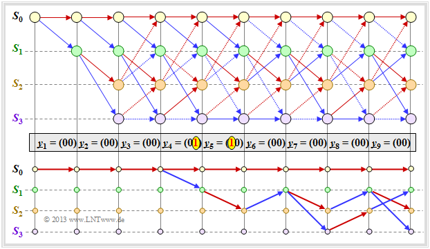
The graphic shows in the upper part an exemplary trellis for

• "our standard encoder"  $(R = 1/2, \ m = 2)$

$$ {\rm G}(D) = (1 + D + D^2, \ 1 + D^2),$$

• the zero input sequence   ⇒   $\underline{u} = \underline{0} = (0, 0, 0, \ \text{...})$;  output:

$$\underline{x} = \underline{0} = (00, 00, 00, \ \text{...}),$$

• in each case,  transmission errors at  $i = 4$  and  $i = 5$.

⇒   Based on the stroke types,  one can recognize allowed  $($solid$)$  and forbidden  $($dotted$)$  arrows in red  $(u_i = 0)$  and blue  $(u_i = 1)$.

Dotted lines have lost a comparison against a competitor and cannot be part of the selected path.

⇒   The lower part of the graph shows the  $2^m = 4$  surviving paths  ${\it \Phi}_9(S_{\mu})$  at time  $i = 9$.

• It is easiest to find these paths from right to left  $($"backward"$)$.

• The following specification shows the traversed states  $S_{\mu}$  but in the forward direction:
  

$${\it \Phi}_9(S_0) \text{:} \hspace{0.4cm} S_0 → S_0 → S_0 → S_0 → S_0 → S_0 → S_0 → S_0 → S_0 → S_0,$$

$${\it \Phi}_9(S_1) \text{:} \hspace{0.4cm} S_0 → S_0 → S_0 → S_0 → S_1 → S_2 → S_1 → S_3 → S_2 → S_1,$$

$${\it \Phi}_9(S_2) \text{:} \hspace{0.4cm} S_0 → S_0 → S_0 → S_0 → S_1 → S_2 → S_1 → S_2 → S_1 → S_2,$$

$${\it \Phi}_9(S_3) \text{:} \hspace{0.4cm} S_0 → S_0 → S_0 → S_0 → S_1 → S_2 → S_1 → S_2 → S_1 → S_3.$$

At earlier times  $(i<9)$  other survivors  ${\it \Phi}_i(S_{\mu})$  would result. Therefore, we define:

$\text{Definition:}$  The   »survivor«   ${\it \Phi}_i(S_{\mu})$  is the continuous path from the start  $S_0$  $($at  $i = 0)$  to the node  $S_{\mu}$ at time  $i$.

• It is recommended to search for paths in the backward direction

.

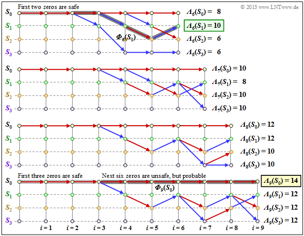
The following graph shows the surviving paths for time points  $i = 6$  to  $i = 9$.  In addition,  the respective metrics  $($accumulated correlaltion values$)$  ${\it \Lambda}_i(S_{\mu})$  for all four states are given.

The survivors  ${\it \Phi}_6, \ \text{...} \ , \ {\it \Phi}_9$

This graph is to be interpreted as follows:

1. At time  $i = 9$  no final maximum likelihood decision can yet be made about the first nine bits of the information sequence.
2. But it is already certain that the most probable bit sequence is represented by one of the paths  ${\it \Phi}_9(S_0), \ \text{...} \ , \ {\it \Phi}_9(S_3)$.
   
3. Since all four paths up to  $i = 3$  are identical,  the decision  "$v_1 = 0,\ v_2 = 0, \ v_3 = 0$"  is the the most probable.  Also at a later time no other decision would be made. 
4. Regarding the bits  $v_4, \ v_5, \ \text{...}$  one should not decide at this early stage.  Only the forst two zeros are safe,  not  $v_3 = 0$.
5. If one had to make a constraint decision at time  $i = 9$  one would choose  ${\it \Phi}_9(S_0)$   ⇒   $\underline{v} = (0, 0, \text{. ..} \ , 0)$ since the metric  ${\it \Lambda}_9(S_0) = 14$  is larger than the comparison metrics.
   
6. The forced decision at time  $i = 9$  leads to the correct result in this example,  see lower sketch.
7. A decision at time  $i = 6$  would have would have led to the wrong result  ⇒   $\underline{v} = (0, 0, 0, 1, 0, 1)$,  see upper sketch.
8. At time  $i = 7$  resp.  $i = 8$,  a forced decision would not have been clear,  as shown in the two middle diagrams
   

Other decoding methods for convolutional codes

We have so far dealt only with the Viterbi algorithm in the form presented in 1967 by Andrew J. Viterbi in  [Vit67].  It was not until 1974 that  $\text{George David Forney}$  proved that this algorithm performs maximum likelihood decoding of convolutional codes.

But even in the years before,  many scientists were very eager to provide efficient decoding methods for the convolutional codes first described by  $\text{Peter Elias}$  in 1955.  Among others,  more detailed descriptions can be found for example in  [Bos99].

• $\text{Sequential Decoding}$   by J. M. Wozencraft and B. Reiffen from 1961,
  

• the proposal of  $\text{Robert Mario Fano}$  (1963),  which became known as the  "Fano algorithm",
  

• the work of Kamil Zigangirov  (1966)  and  $\text{Frederick Jelinek}$  (1969),  whose decoding method is also referred to as the  "stack algorithm".
  
  

All of these decoding schemes,  as well as the Viterbi algorithm as described so far,  provide  "hard decided"  output values   ⇒   $v_i ∈ \{0, 1\}$.  Often,  however,  information about the reliability of the decisions made would be desirable,  especially when there is a concatenated coding scheme with an outer and an inner code.

If the reliability of the bits decided by the inner decoder is known at least roughly,  this information can be used to  (significantly)  reduce the bit error probability of the outer decoder.  The  "soft output Viterbi algorithm"  $\rm(SOVA)$  proposed by  $\text{Joachim Hagenauer}$  in  [Hag90]  allows to specify a reliability measure in each case in addition to the decided symbols.

Finally, we go into some detail about the  »BCJR algorithm«  named after its inventors L. R. Bahl, J. Cocke, F. Jelinek, and J. Raviv  [BCJR74].

While the Viterbi algorithm only estimates the total sequence   ⇒   $\text{block-wise ML}$,  the BCJR algorithm estimates a single bit considering the entire received sequence.  So this is a  "bit-wise maximum a posteriori decoding"   ⇒   $\text{bit-wise MAP}$.

$\text{Conclusion:}$ 

The difference between Viterbi–algorithm and BCJR algorithm shall be  – greatly simplified –  illustrated by the example of a terminated convolutional code:

• The   »Viterbi algorithm «  processes the trellis in only one direction  – the forward direction  – and computes the metrics  ${\it \Lambda}_i(S_{\mu})$  for each node.  After reaching the terminal node,  the surviving path is searched,  which identifies the most probable code sequence.
  

• In the   »BCJR algorithm «  the trellis is processed twice,  once in forward direction and then in backward direction.  Two metrics can then be specified for each node,  from which the aposterori probability can be determined for each bit

.

Hints:

1.   This short summary is based on the textbook  [Bos99].
2.   A description of the BCJR–algorithm follows also in section  "Hard Decision vs. Soft Decision"  "in the fourth main chapter"  "Iterative Decoding Methods".
   

Exercises for the chapter

Exercise 3.09: Basics of the Viterbi Algorithm

Exercise 3.09Z: Viterbi Algorithm again

Exercise 3.10: Metric Calculation

Exercise 3.10Z: Maximum Likelihood Decoding of Convolutional Codes

Exercise 3.11: Viterbi Path Finding

References

- ↑ Viterbi, A.J.: Error Bounds for Convolutional Codes and an Asymptotically Optimum Decoding Algorithm. In: IEEE Transactions on Information Theory, vol. IT-13, pp. 260-269, April 1967.
- ↑ 2.0 2.1 Bossert, M.: Channel Coding for Telecommunications. Wiley & Sons, 1999.
- ↑ Hagenauer, J.: Soft Output Viterbi Decoder. In: Technischer Report, Deutsche Forschungsanstalt für Luft- und Raumfahrt (DLR), 1990.
- ↑ Bahl, L.R.; Cocke, J.; Jelinek, F.; Raviv, J.: Optimal Decoding of Linear Codes for Minimizing Symbol Error Rate. In: IEEE Transactions on Information Theory, Vol. IT-20, pp. 284-287, 1974.