Difference between revisions of "Channel Coding/Algebraic and Polynomial Description"
| (14 intermediate revisions by 2 users not shown) | |||
| Line 13: | Line 13: | ||
# Therefore, the generator matrix $\mathbf{G}$ will also be infinitely extended in both directions.<br><br> | # Therefore, the generator matrix $\mathbf{G}$ will also be infinitely extended in both directions.<br><br> | ||
| − | In preparation for the introduction of the generator matrix $\mathbf{G}$ | + | In preparation for the introduction of the generator matrix $\mathbf{G}$ in the next section, |
*we define $m + 1$ "partial matrices", each with $k$ rows and $n$ columns, which we denote by $\mathbf{G}_l$ | *we define $m + 1$ "partial matrices", each with $k$ rows and $n$ columns, which we denote by $\mathbf{G}_l$ | ||
| Line 99: | Line 99: | ||
*The generator matrix $\mathbf{G}$ actually extends downwards and to the right to infinity. Explicitly shown, however, are only eight rows and twelve columns. | *The generator matrix $\mathbf{G}$ actually extends downwards and to the right to infinity. Explicitly shown, however, are only eight rows and twelve columns. | ||
| − | *For the temporal information sequence $\underline{u} = (0, 1, 1, 0, 0, 0, 1, 1)$ the drawn matrix part is sufficient. The | + | *For the temporal information sequence $\underline{u} = (0, 1, 1, 0, 0, 0, 1, 1)$ the drawn matrix part is sufficient. The encoded sequence is then: |
:$$\underline{x} = (0, 1, 1, 0, 0, 1, 1, 1, 1, 1, 1, 0).$$ | :$$\underline{x} = (0, 1, 1, 0, 0, 1, 1, 1, 1, 1, 1, 0).$$ | ||
| Line 136: | Line 136: | ||
\end{pmatrix}\hspace{0.05cm}.$$ | \end{pmatrix}\hspace{0.05cm}.$$ | ||
| − | *For the input sequence $\underline{u} = (1, 0, 1, 1)$, the | + | *For the input sequence $\underline{u} = (1, 0, 1, 1)$, the encoded sequence starts with $\underline{x} = (1, 1, 0, 1, 1, 1, 1, 0, \ \text{...})$. |
*This result is equal to the sum of rows '''1''', '''3''' and '''4''' of the generator matrix.<br><br> | *This result is equal to the sum of rows '''1''', '''3''' and '''4''' of the generator matrix.<br><br> | ||
| Line 165: | Line 165: | ||
\end{pmatrix}\hspace{0.05cm}.</math> | \end{pmatrix}\hspace{0.05cm}.</math> | ||
| − | *Here the input sequence $\underline{u} = (1, 0, 1, 1)$ leads to the | + | *Here the input sequence $\underline{u} = (1, 0, 1, 1)$ leads to the encoded sequence $\underline{x} = (1, 1, 1, 0, 0, 0, 0, 1, \ \text{...})$.<br><br> |
[[File:P ID2604 KC T 3 2 S3c.png|right|frame|Convolutional encoder $(k = 1, \ n = 3, \ m = 3)$]] | [[File:P ID2604 KC T 3 2 S3c.png|right|frame|Convolutional encoder $(k = 1, \ n = 3, \ m = 3)$]] | ||
| Line 195: | Line 195: | ||
\end{pmatrix}\hspace{0.05cm}.</math> | \end{pmatrix}\hspace{0.05cm}.</math> | ||
| − | *One obtains for $\underline{u} = (1, 0, 1, 1)$ the | + | *One obtains for $\underline{u} = (1, 0, 1, 1)$ the encoded sequence $\underline{x} = (1, 1, 0, 0, 0, 1, 1, 1, 1, 1, 0, 0, \ \text{...})$.<br> |
== GF(2) description forms of a digital filter == | == GF(2) description forms of a digital filter == | ||
| Line 221: | Line 221: | ||
::<math>\underline{x} = \underline{u} * \underline{g}\hspace{0.05cm}.</math> | ::<math>\underline{x} = \underline{u} * \underline{g}\hspace{0.05cm}.</math> | ||
| − | *Major difference compared to the chapter »[[Theory_of_Stochastic_Signals/Digital_Filters| | + | *Major difference compared to the chapter »[[Theory_of_Stochastic_Signals/Digital_Filters|"Digital Filters"]]« in the book "Theory of Stochastic Signals" is the modulo-2 addition $(1 + 1 = 0)$ instead of the conventional addition $(1 + 1 = 2)$.<br><br> |
{{GraueBox|TEXT= | {{GraueBox|TEXT= | ||
| Line 254: | Line 254: | ||
X(D) = \sum_{i = 0}^{\infty} x_i \cdot D\hspace{0.05cm}^i \hspace{0.05cm}.</math>}}<br> | X(D) = \sum_{i = 0}^{\infty} x_i \cdot D\hspace{0.05cm}^i \hspace{0.05cm}.</math>}}<br> | ||
| − | <u>Note</u>: In the literature, sometimes $x(D)$ is used instead of $X(D)$. However, we write in our learning tutorial all image domain functions ⇒ "spectral domain functions" with capital letters,  | + | <u>Note</u>: In the literature, sometimes $x(D)$ is used instead of $X(D)$. However, we write in our learning tutorial all image domain functions ⇒ "spectral domain functions" with capital letters, for example the Fourier transform, the Laplace transform and the D–transform: |
::<math>x(t) \hspace{0.15cm} | ::<math>x(t) \hspace{0.15cm} | ||
| Line 281: | Line 281: | ||
{{BlaueBox|TEXT= | {{BlaueBox|TEXT= | ||
| − | $\text{Theorem:}$ As with all spectral transformations, the <b>multiplication</b> applies to the D–transform in the image domain, since the $($discrete$)$ time | + | $\text{Theorem:}$ As with all spectral transformations, the »<b>multiplication</b>« applies to the D–transform in the image domain, since the $($discrete$)$ time functions $\underline{u}$ and $\underline{g}$ are interconnected by the »<b>convolution</b>«: |
::<math>\underline{x} = \underline{u} * \underline{g} \quad | ::<math>\underline{x} = \underline{u} * \underline{g} \quad | ||
| Line 287: | Line 287: | ||
X(D) = U(D) \cdot G(D) \hspace{0.05cm}.</math> | X(D) = U(D) \cdot G(D) \hspace{0.05cm}.</math> | ||
| − | *The $($rather simple$)$ $\rm proof$ of this important result can be found in the specification for [[Aufgaben:Exercise_3.3Z:_Convolution_and_D-Transformation| | + | *The $($rather simple$)$ $\rm proof$ of this important result can be found in the specification for [[Aufgaben:Exercise_3.3Z:_Convolution_and_D-Transformation|"Exercise 3.3Z"]]. |
| − | *As in »[[Linear_and_Time_Invariant_Systems/System_Description_in_Frequency_Domain#Frequency_response_.E2.80. 93_Transfer_function|$\text{system theory}$]]« commonly, the D–transform $G(D)$ of the impulse response $\underline{g}$ is also called "transfer function".}} | + | *As in »[[Linear_and_Time_Invariant_Systems/System_Description_in_Frequency_Domain#Frequency_response_.E2.80.93_Transfer_function|$\text{system theory}$]]« commonly, the D–transform $G(D)$ of the impulse response $\underline{g}$ is also called "transfer function".}} |
| Line 305: | Line 305: | ||
G(D) = 1+ D^2 + D^3 \hspace{0.05cm}.</math> | G(D) = 1+ D^2 + D^3 \hspace{0.05cm}.</math> | ||
| − | *As in $\text{Example 3}$ $($ | + | *As in $\text{Example 3}$ $($in this section above$)$, you get also on this solution path: |
::<math>X(D) = U(D) \cdot G(D) = (1+D) \cdot (1+ D^2 + D^3) </math> | ::<math>X(D) = U(D) \cdot G(D) = (1+D) \cdot (1+ D^2 + D^3) </math> | ||
| Line 319: | Line 319: | ||
== Application of the D–transform to rate $1/n$ convolution encoders == | == Application of the D–transform to rate $1/n$ convolution encoders == | ||
<br> | <br> | ||
| − | We now apply the results of the last | + | We now apply the results of the last section to a convolutional encoder, restricting ourselves for the moment to the special case $k = 1$. |
*Such a $(n, \ k = 1)$ convolutional code can be realized with $n$ digital filters operating in parallel on the same information sequence $\underline{u}$. | *Such a $(n, \ k = 1)$ convolutional code can be realized with $n$ digital filters operating in parallel on the same information sequence $\underline{u}$. | ||
| Line 328: | Line 328: | ||
The following equations apply equally to both filters, setting $j = 1$ for the upper filter and $j = 2$ for the lower filter: | The following equations apply equally to both filters, setting $j = 1$ for the upper filter and $j = 2$ for the lower filter: | ||
| − | *The <b>impulse responses</b> of the two filters result in | + | *The »<b>impulse responses</b>« of the two filters result in |
::<math>\underline{g}^{(j)} = (g_0^{(j)}, g_1^{(j)}, \hspace{0.05cm}\text{...}\hspace{0.05cm}, g_m^{(j)}\hspace{0.01cm}) \hspace{0.05cm},\hspace{0.2cm}{\rm with }\hspace{0.15cm} j \in \{1,2\}\hspace{0.05cm}.</math> | ::<math>\underline{g}^{(j)} = (g_0^{(j)}, g_1^{(j)}, \hspace{0.05cm}\text{...}\hspace{0.05cm}, g_m^{(j)}\hspace{0.01cm}) \hspace{0.05cm},\hspace{0.2cm}{\rm with }\hspace{0.15cm} j \in \{1,2\}\hspace{0.05cm}.</math> | ||
| − | *The two <b>output sequences</b> are as follows, considering that both filters operate on the same input sequence $\underline{u} = (u_0, u_1, u_2, \hspace{0.05cm} \text{...})$ : | + | *The two »<b>output sequences</b>« are as follows, considering that both filters operate on the same input sequence $\underline{u} = (u_0, u_1, u_2, \hspace{0.05cm} \text{...})$ : |
::<math>\underline{x}^{(j)} = (x_0^{(j)}, x_1^{(j)}, x_2^{(j)}, \hspace{0.05cm}\text{...}\hspace{0.05cm}) = \underline{u} \cdot \underline{g}^{(j)} \hspace{0.05cm},\hspace{0.2cm}{\rm with }\hspace{0.15cm} j \in \{1,2\}\hspace{0.05cm}.</math> | ::<math>\underline{x}^{(j)} = (x_0^{(j)}, x_1^{(j)}, x_2^{(j)}, \hspace{0.05cm}\text{...}\hspace{0.05cm}) = \underline{u} \cdot \underline{g}^{(j)} \hspace{0.05cm},\hspace{0.2cm}{\rm with }\hspace{0.15cm} j \in \{1,2\}\hspace{0.05cm}.</math> | ||
| − | *For the <b>D–transform</b> of the output sequences: | + | *For the »<b>D–transform</b>« of the output sequences: |
::<math>X^{(j)}(D) = U(D) \cdot G^{(j)}(D) \hspace{0.05cm},\hspace{0.2cm}{\rm with }\hspace{0.15cm} j \in \{1,2\}\hspace{0.05cm}.</math> | ::<math>X^{(j)}(D) = U(D) \cdot G^{(j)}(D) \hspace{0.05cm},\hspace{0.2cm}{\rm with }\hspace{0.15cm} j \in \{1,2\}\hspace{0.05cm}.</math> | ||
| Line 347: | Line 347: | ||
::<math>\underline{G}(D) = \left ( G^{(1)}(D), G^{(2)}(D), \hspace{0.05cm}\text{...}\hspace{0.1cm}, G^{(n)} (D) \right )\hspace{0.05cm}.</math> | ::<math>\underline{G}(D) = \left ( G^{(1)}(D), G^{(2)}(D), \hspace{0.05cm}\text{...}\hspace{0.1cm}, G^{(n)} (D) \right )\hspace{0.05cm}.</math> | ||
| − | *The vector $\underline{X}(D)$ contains the D–transform of $n$ | + | *The vector $\underline{X}(D)$ contains the D–transform of $n$ encoded sequences $\underline{x}^{(1)}, \underline{x}^{(2)}, \ \text{...} \ , \underline{x}^{(n)}$: |
::<math>\underline{X}(D) = \left ( X^{(1)}(D), X^{(2)}(D), \hspace{0.05cm}\text{...}\hspace{0.1cm}, X^{(n)} (D) \right )\hspace{0.05cm}.</math> | ::<math>\underline{X}(D) = \left ( X^{(1)}(D), X^{(2)}(D), \hspace{0.05cm}\text{...}\hspace{0.1cm}, X^{(n)} (D) \right )\hspace{0.05cm}.</math> | ||
| Line 382: | Line 382: | ||
::<math>\Rightarrow \underline{x}^{(2)} = (\hspace{0.05cm}1\hspace{0.05cm},\hspace{0.05cm}0\hspace{0.05cm},\hspace{0.05cm} 0\hspace{0.05cm},\hspace{0.05cm} 1\hspace{0.05cm},\hspace{0.05cm} 1\hspace{0.05cm},\hspace{0.05cm} 1\hspace{0.05cm},\hspace{0.05cm} 0\hspace{0.05cm}, \hspace{0.05cm} 0\hspace{0.05cm}, \hspace{0.05cm} \text{...} \hspace{0.05cm} \hspace{0.05cm}) \hspace{0.05cm}.</math> | ::<math>\Rightarrow \underline{x}^{(2)} = (\hspace{0.05cm}1\hspace{0.05cm},\hspace{0.05cm}0\hspace{0.05cm},\hspace{0.05cm} 0\hspace{0.05cm},\hspace{0.05cm} 1\hspace{0.05cm},\hspace{0.05cm} 1\hspace{0.05cm},\hspace{0.05cm} 1\hspace{0.05cm},\hspace{0.05cm} 0\hspace{0.05cm}, \hspace{0.05cm} 0\hspace{0.05cm}, \hspace{0.05cm} \text{...} \hspace{0.05cm} \hspace{0.05cm}) \hspace{0.05cm}.</math> | ||
| − | *We got the same result in [[Aufgaben:Exercise_3.1Z:_Convolution_Codes_of_Rate_1/2| | + | *We got the same result in [[Aufgaben:Exercise_3.1Z:_Convolution_Codes_of_Rate_1/2|"Exercise 3.1Z"]] on other way. After multiplexing the two strands, you get again: |
:$$\underline{x} = (11, 10, 00, 01, 01, 11, 00, 00, \hspace{0.05cm} \text{...} \hspace{0.05cm}).$$}}<br> | :$$\underline{x} = (11, 10, 00, 01, 01, 11, 00, 00, \hspace{0.05cm} \text{...} \hspace{0.05cm}).$$}}<br> | ||
| Line 394: | Line 394: | ||
Now we extend the result to convolutional encoders with more than one input ⇒ $k ≥ 2$ $($see graph$)$.<br> | Now we extend the result to convolutional encoders with more than one input ⇒ $k ≥ 2$ $($see graph$)$.<br> | ||
| − | In order to map a convolutional code of rate $k/n$ in the D& | + | In order to map a convolutional code of rate $k/n$ in the D–domain, the dimension of the above vector equation must be increased with respect to input and transfer function: |
::<math>\underline{X}(D) = \underline{U}(D) \cdot { \boldsymbol{\rm G}}(D)\hspace{0.05cm}.</math> | ::<math>\underline{X}(D) = \underline{U}(D) \cdot { \boldsymbol{\rm G}}(D)\hspace{0.05cm}.</math> | ||
| Line 413: | Line 413: | ||
*Each of the $k \cdot n$ matrix elements $G_i^{(j)}(D)$ with $1 ≤ i ≤ k,\ 1 ≤ j ≤ n$ is a polynomial over the dummy variable $D$ in the Galois field ${\rm GF}(2)$, maximal of degree $m$, where $m$ denotes the memory.<br> | *Each of the $k \cdot n$ matrix elements $G_i^{(j)}(D)$ with $1 ≤ i ≤ k,\ 1 ≤ j ≤ n$ is a polynomial over the dummy variable $D$ in the Galois field ${\rm GF}(2)$, maximal of degree $m$, where $m$ denotes the memory.<br> | ||
| − | *For the above transfer function matrix, using the [[Channel_Coding/Algebraic_and_Polynomial_Description#Division_of_the_generator_matrix_into_partial_matrices| $\text{partial matrices}$]] $\mathbf{G}_0, \ \text{...} \ , \mathbf{G}_m$ also be written $($as index we use again $l)$: | + | *For the above transfer function matrix, using the [[Channel_Coding/Algebraic_and_Polynomial_Description#Division_of_the_generator_matrix_into_partial_matrices| »$\text{partial matrices}$«]] $\mathbf{G}_0, \ \text{...} \ , \mathbf{G}_m$ also be written $($as index we use again $l)$: |
::<math>{\boldsymbol{\rm G}}(D) = \sum_{l = 0}^{m} {\boldsymbol{\rm G}}_l \cdot D\hspace{0.03cm}^l | ::<math>{\boldsymbol{\rm G}}(D) = \sum_{l = 0}^{m} {\boldsymbol{\rm G}}_l \cdot D\hspace{0.03cm}^l | ||
| Line 460: | Line 460: | ||
\end{pmatrix}\hspace{0.05cm}.</math> | \end{pmatrix}\hspace{0.05cm}.</math> | ||
| − | *This results in the following | + | *This results in the following encoded sequences in the three strands: |
::<math>{X}^{(1)}(D) = (D + D^3) \cdot (1+D) + (1 + D^3) \cdot D =D + D^2 + D^3 + D^4 + D + D^4 = D^2 + D^3</math> | ::<math>{X}^{(1)}(D) = (D + D^3) \cdot (1+D) + (1 + D^3) \cdot D =D + D^2 + D^3 + D^4 + D + D^4 = D^2 + D^3</math> | ||
| Line 475: | Line 475: | ||
We have already obtained the same results in other ways in previous examples: | We have already obtained the same results in other ways in previous examples: | ||
| − | * in [[Channel_Coding/Basics_of_Convolutional_Coding#Convolutional_encoder_with_two_inputs|$\text{Example 4}$]] the chapter "Basics of Convolutional Coding",<br> | + | * in [[Channel_Coding/Basics_of_Convolutional_Coding#Convolutional_encoder_with_two_inputs|$\text{Example 4}$]] of the chapter "Basics of Convolutional Coding",<br> |
| − | *in [[Channel_Coding/Algebraic_and_Polynomial_Description# | + | *in [[Channel_Coding/Algebraic_and_Polynomial_Description#Generator_matrix_of_a_convolutional_encoder_with_memory_.7F.27.22.60UNIQ-MathJax64-QINU.60.22.27.7F| $\text{Example 2}$]] of the current chapter.}}<br> |
== Systematic convolutional codes == | == Systematic convolutional codes == | ||
| Line 484: | Line 484: | ||
[[File:P ID2611 KC T 3 2 S7 v2.png|right|frame|Systematic convolutional code with $k = 3, \ n = 4$|class=fit]] | [[File:P ID2611 KC T 3 2 S7 v2.png|right|frame|Systematic convolutional code with $k = 3, \ n = 4$|class=fit]] | ||
| − | * | + | *This $k × n$ matrix is used to recognize whether it is a [[Channel_Coding/General_Description_of_Linear_Block_Codes#Systematic_Codes| »$\text{systematic code}$«]]. |
| − | *This refers to a code where the | + | *This refers to a code where the encoded sequences $\underline{x}^{(1)}, \ \text{...} \ , \ \underline{x}^{(k)}$ are identical with the information sequences $\underline{u}^{(1)}, \ \text{...} \ , \ \underline{u}^{(k)}$. |
*The graph shows an example of a systematic $(n = 4, \ k = 3)$ convolutional code.<br> | *The graph shows an example of a systematic $(n = 4, \ k = 3)$ convolutional code.<br> | ||
| Line 531: | Line 531: | ||
{{GraueBox|TEXT= | {{GraueBox|TEXT= | ||
$\text{Example 8:}$ | $\text{Example 8:}$ | ||
| − | The | + | The encoder of rate $2/3$ considered often in the last sections is not systematic because e.g. $\underline{x}^{(1)} ≠ \underline{u}^{(1)}, \ \underline{x}^{(2)} ≠ \underline{u}^{(2)}$ holds $($see adjacent graphic$)$.<br> |
[[File:P ID2613 KC T 3 2 S1 neu.png|right|frame|Convolutional encoder of rate $2/3$]] | [[File:P ID2613 KC T 3 2 S1 neu.png|right|frame|Convolutional encoder of rate $2/3$]] | ||
| Line 599: | Line 599: | ||
* The coefficients $b_1, \ \text{...} \ , \ b_m$ form a feedback branch. | * The coefficients $b_1, \ \text{...} \ , \ b_m$ form a feedback branch. | ||
| − | *All coefficients are binary, so $1$ $($continuous connection$)$ or $0$ $($missing connection$)$. | + | *All coefficients are binary, |
| + | :*so $1$ $($continuous connection$)$ | ||
| + | :*or $0$ $($missing connection$)$. | ||
<br clear=all> | <br clear=all> | ||
{{GraueBox|TEXT= | {{GraueBox|TEXT= | ||
Latest revision as of 19:50, 2 December 2022
Contents
- 1 Division of the generator matrix into partial matrices
- 2 Generator matrix of a convolutional encoder with memory $m$
- 3 Generator matrix for convolutional encoder of rate $1/n$
- 4 GF(2) description forms of a digital filter
- 5 Application of the D–transform to rate $1/n$ convolution encoders
- 6 Transfer Function Matrix
- 7 Systematic convolutional codes
- 8 Equivalent systematic convolutional code
- 9 Filter structure with fractional–rational transfer function
- 10 Exercises for the chapter
Division of the generator matrix into partial matrices
Following the discussion in the earlier section "Linear Codes and Cyclic Codes" the code word $\underline{x}$ of a linear block code can be determined from the information word $\underline{u}$ and the generator matrix $\mathbf{G}$ in a simple way: $\underline{x} = \underline{u} \cdot { \boldsymbol{\rm G}}$. The following holds:
- The vectors $\underline{u}$ and $\underline{x}$ have length $k$ $($bit count of an info word$)$ resp. $n$ $($bit count of a code word$)$ and $\mathbf{G}$ has dimension $k × n$ $(k$ rows and $n$ columns$)$.
- In convolutional coding, on the other hand $\underline{u}$ and $\underline{x}$ denote sequences with $k\hspace{0.05cm}' → ∞$ and $n\hspace{0.05cm}' → ∞$.
- Therefore, the generator matrix $\mathbf{G}$ will also be infinitely extended in both directions.
In preparation for the introduction of the generator matrix $\mathbf{G}$ in the next section,
- we define $m + 1$ "partial matrices", each with $k$ rows and $n$ columns, which we denote by $\mathbf{G}_l$
- where $0 ≤ l ≤ m$ holds.
$\text{Definition:}$ The »partial matrix« $\mathbf{G}_l$ describes the following fact:
- If the matrix element $\mathbf{G}_l(\kappa, j) = 1$, this says that the code bit $x_i^{(j)}$ is influenced by the information bit $u_{i-l}^{(\kappa)}$.
- Otherwise, this matrix element is $\mathbf{G}_l(\kappa, j) =0$.
This definition will now be illustrated by an example.
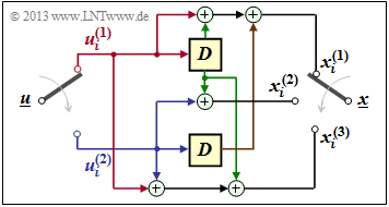
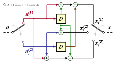
$\text{Example 1:}$ We again consider the convolutional encoder according to the diagram with the following code bits:
- \[x_i^{(1)} = u_{i}^{(1)} + u_{i-1}^{(1)}+ u_{i-1}^{(2)} \hspace{0.05cm},\]
- \[x_i^{(2)} = u_{i}^{(2)} + u_{i-1}^{(1)} \hspace{0.05cm},\]
- \[x_i^{(3)} = u_{i}^{(1)} + u_{i}^{(2)}+ u_{i-1}^{(1)} \hspace{0.05cm}.\]
Because of the memory $m = 1$ this encoder is fully characterized by the partial matrices $\mathbf{G}_0$ and $\mathbf{G}_1$ :
- \[{ \boldsymbol{\rm G} }_0 = \begin{pmatrix} 1 & 0 & 1\\ 0 & 1 & 1 \end{pmatrix} \hspace{0.05cm}, \hspace{0.5cm} { \boldsymbol{\rm G} }_1 = \begin{pmatrix} 1 & 1 & 1\\ 1 & 0 & 0 \end{pmatrix}\hspace{0.05cm}.\]
These matrices are to be interpreted as follows:
- First row of $\mathbf{G}_0$, red arrows: $\hspace{1.3cm}u_i^{(1)}$ affects both $x_i^{(1)}$ and $x_i^{(3)}$, but not $x_i^{(2)}$.
- Second row of $\mathbf{G}_0$, blue arrows: $\hspace{0.6cm}u_i^{(2)}$ affects $x_i^{(2)}$ and $x_i^{(3)}$, but not $x_i^{(1)}$.
- First row of $\mathbf{G}_1$, green arrows: $\hspace{0.9cm}u_{i-1}^{(1)}$ affects all three encoder outputs.
- Second row of $\mathbf{G}_1$, brown arrow: $\hspace{0.45cm}u_{i-1}^{(2)}$ affects only $x_i^{(1)}$.
Generator matrix of a convolutional encoder with memory $m$
The $n$ code bits at time $i$ can be expressed with the partial matrices $\mathbf{G}_0, \hspace{0.05cm} \text{...} \hspace{0.05cm} , \mathbf{G}_m$ as follows:
- \[\underline{x}_i = \sum_{l = 0}^{m} \hspace{0.15cm}\underline{u}_{i-l} \cdot { \boldsymbol{\rm G}}_l = \underline{u}_{i} \cdot { \boldsymbol{\rm G}}_0 + \underline{u}_{i-1} \cdot { \boldsymbol{\rm G}}_1 +\hspace{0.05cm} \text{...} \hspace{0.05cm} + \underline{u}_{i-m} \cdot { \boldsymbol{\rm G}}_m \hspace{0.05cm}.\]
- The following vectorial quantities must be taken into account:
- \[\underline{\it u}_i = \left ( u_i^{(1)}, u_i^{(2)}, \hspace{0.05cm}\text{...} \hspace{0.1cm}, u_i^{(k)}\right )\hspace{0.05cm},\hspace{0.5cm} \underline{\it x}_i = \left ( x_i^{(1)}, x_i^{(2)}, \hspace{0.05cm}\text{...} \hspace{0.1cm}, x_i^{(n)}\right )\hspace{0.05cm}.\]
- Considering the sequences
- \[\underline{\it u} = \big( \underline{\it u}_1\hspace{0.05cm}, \underline{\it u}_2\hspace{0.05cm}, \hspace{0.05cm}\text{...} \hspace{0.1cm}, \underline{\it u}_i\hspace{0.05cm}, \hspace{0.05cm}\text{...} \hspace{0.1cm} \big)\hspace{0.05cm},\hspace{0.5cm} \underline{\it x} = \big( \underline{\it x}_1\hspace{0.05cm}, \underline{\it x}_2\hspace{0.05cm}, \hspace{0.05cm}\text{...} \hspace{0.1cm}, \underline{\it x}_i\hspace{0.05cm}, \hspace{0.05cm}\text{...} \hspace{0.1cm} \big)\hspace{0.05cm},\]
- starting at $i = 1$ and extending in time to infinity, this relation can be expressed by the matrix equation $\underline{x} = \underline{u} \cdot \mathbf{G}$. Here, holds for the generator matrix:
- \[{ \boldsymbol{\rm G}}=\begin{pmatrix} { \boldsymbol{\rm G}}_0 & { \boldsymbol{\rm G}}_1 & { \boldsymbol{\rm G}}_2 & \cdots & { \boldsymbol{\rm G}}_m & & & \\ & { \boldsymbol{\rm G}}_0 & { \boldsymbol{\rm G}}_1 & { \boldsymbol{\rm G}}_2 & \cdots & { \boldsymbol{\rm G}}_m & &\\ & & { \boldsymbol{\rm G}}_0 & { \boldsymbol{\rm G}}_1 & { \boldsymbol{\rm G}}_2 & \cdots & { \boldsymbol{\rm G}}_m &\\ & & & \cdots & \cdots & & & \cdots \end{pmatrix}\hspace{0.05cm}.\]
- From this equation one immediately recognizes the memory $m$ of the convolutional code.
- The parameters $k$ and $n$ are not directly readable.
- However, they are determined by the number of rows and columns of the partial matrices $\mathbf{G}_l$.
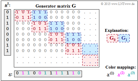
$\text{Example 2:}$ With the two matrices $\mathbf{G}_0$ and $\mathbf{G}_1$ – see $\text{Example 1}$ – the matrix sketched on the right $\mathbf{G}$ is obtained.
It should be noted:
- The generator matrix $\mathbf{G}$ actually extends downwards and to the right to infinity. Explicitly shown, however, are only eight rows and twelve columns.
- For the temporal information sequence $\underline{u} = (0, 1, 1, 0, 0, 0, 1, 1)$ the drawn matrix part is sufficient. The encoded sequence is then:
- $$\underline{x} = (0, 1, 1, 0, 0, 1, 1, 1, 1, 1, 1, 0).$$
- On the basis of the label colors, the $n = 3$ code word strings can be read.
- We got the same result $($in a different way$)$ in the $\text{Example 4}$ at the end of the last chapter:
- $$\underline{\it x}^{(1)} = (0\hspace{0.05cm}, 0\hspace{0.05cm}, 1\hspace{0.05cm}, 1) \hspace{0.05cm},$$
- $$\underline{\it x}^{(2)} = (1\hspace{0.05cm}, 0\hspace{0.05cm},1\hspace{0.05cm}, 1) \hspace{0.05cm},$$
- $$ \underline{\it x}^{(3)} = (1\hspace{0.05cm}, 1\hspace{0.05cm}, 1\hspace{0.05cm}, 0) \hspace{0.05cm}.$$
Generator matrix for convolutional encoder of rate $1/n$
We now consider the special case $k = 1$,
- on the one hand for reasons of simplest possible representation,
- but also because convolutional encoders of rate $1/n$ have great importance for practice.
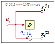
Convolutional encoder with $k = 1, \ n = 2, \ m = 1$
- From the adjacent sketch can be derived:
- $${ \boldsymbol{\rm G}}_0=\begin{pmatrix} 1 & 1 \end{pmatrix}\hspace{0.05cm},\hspace{0.3cm} { \boldsymbol{\rm G}}_1=\begin{pmatrix} 0 & 1 \end{pmatrix}\hspace{0.3cm} \Rightarrow \hspace{0.3cm}$$
- Thus, the resulting generator matrix is:
- $${ \boldsymbol{\rm G}}=\begin{pmatrix} 11 & 01 & 00 & 00 & 00 & \cdots & \\ 00 & 11 & 01 & 00 & 00 & \cdots & \\ 00 & 00 & 11 & 01 & 00 & \cdots & \\ 00 & 00 & 00 & 11 & 01 & \cdots & \\ \cdots & \cdots & \cdots & \cdots & \cdots & \cdots \end{pmatrix}\hspace{0.05cm}.$$
- For the input sequence $\underline{u} = (1, 0, 1, 1)$, the encoded sequence starts with $\underline{x} = (1, 1, 0, 1, 1, 1, 1, 0, \ \text{...})$.
- This result is equal to the sum of rows 1, 3 and 4 of the generator matrix.
Convolutional encoder with $k = 1, \ n = 2, \ m = 2$
- Due to the memory order $m = 2$ there are three submatrices here:
- \[{ \boldsymbol{\rm G}}_0=\begin{pmatrix} 1 & 1 \end{pmatrix}\hspace{0.05cm},\hspace{0.3cm} { \boldsymbol{\rm G}}_1=\begin{pmatrix} 1 & 0 \end{pmatrix}\hspace{0.05cm},\hspace{0.3cm} { \boldsymbol{\rm G}}_2=\begin{pmatrix} 1 & 1 \end{pmatrix}\]
- Thus, the resulting generator matrix is now:
- \[ { \boldsymbol{\rm G}}=\begin{pmatrix} 11 & 10 & 11 & 00 & 00 & 00 & \cdots & \\ 00 & 11 & 10 & 11 & 00 & 00 & \cdots & \\ 00 & 00 & 11 & 10 & 11 & 00 & \cdots & \\ 00 & 00 & 00 & 11 & 10 & 11 & \cdots & \\ \cdots & \cdots & \cdots & \cdots & \cdots & \cdots \end{pmatrix}\hspace{0.05cm}.\]
- Here the input sequence $\underline{u} = (1, 0, 1, 1)$ leads to the encoded sequence $\underline{x} = (1, 1, 1, 0, 0, 0, 0, 1, \ \text{...})$.
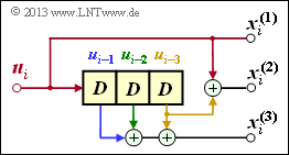
Convolutional encoder with $k = 1, \ n = 3, \ m = 3$
- Because of $m = 3$ there are now four partial matrices of the respective dimension $1 × 3$:
- \[{ \boldsymbol{\rm G}}_0=\begin{pmatrix} 1 & 1 & 0 \end{pmatrix}\hspace{0.05cm},\hspace{0.3cm} { \boldsymbol{\rm G}}_1=\begin{pmatrix} 0 & 0 & 1 \end{pmatrix}\hspace{0.05cm},\hspace{0.3cm} { \boldsymbol{\rm G}}_2=\begin{pmatrix} 0 & 0 & 1 \end{pmatrix}\hspace{0.05cm},\hspace{0.3cm} { \boldsymbol{\rm G}}_3=\begin{pmatrix} 0 & 1 & 1 \end{pmatrix}\hspace{0.05cm}.\]
- Thus, the resulting generator matrix is:
- \[{ \boldsymbol{\rm G}}=\begin{pmatrix} 110 & 001 & 001 & 011 & 000 & 000 & 000 & \cdots & \\ 000 & 110 & 001 & 001 & 011 & 000 & 000 & \cdots & \\ 000 & 000 & 110 & 001 & 001 & 011 & 000 & \cdots & \\ 000 & 000 & 000 & 110 & 001 & 001 & 011 & \cdots & \\ \cdots & \cdots & \cdots & \cdots & \cdots & \cdots & \cdots & \cdots \end{pmatrix}\hspace{0.05cm}.\]
- One obtains for $\underline{u} = (1, 0, 1, 1)$ the encoded sequence $\underline{x} = (1, 1, 0, 0, 0, 1, 1, 1, 1, 1, 0, 0, \ \text{...})$.
GF(2) description forms of a digital filter
In the chapter "Basics of Convolutional Coding" it was already pointed out,
- that a rate $1/n$ convolutional encoder can be realized by several digital filters,
- where the filters operate in parallel with the same input sequence $\underline{u}$ .
Before we elaborate on this statement, we shall first mention the properties of a digital filter for the Galois field ${\rm GF(2)}$.
The graph is to be interpreted as follows:
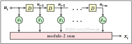
- The filter has impulse response $\underline{g} = (g_0,\ g_1,\ g_2, \ \text{...} \ ,\ g_m)$.
- For all filter coefficients $($with indices $0 ≤ l ≤ m)$ holds: $g_l ∈ {\rm GF}(2) = \{0, 1\}$.
- The individual symbols $u_i$ of the input sequence $\underline{u}$ are also binary: $u_i ∈ \{0, 1\}$.
- Thus, for the output symbol at times $i ≥ 1$ with addition and multiplication in ${\rm GF(2)}$:
- \[x_i = \sum_{l = 0}^{m} g_l \cdot u_{i-l} \hspace{0.05cm}.\]
- This corresponds to the $($discrete time$)$ »$\rm convolution$«, denoted by an asterisk. This can be used to write for the entire output sequence:
- \[\underline{x} = \underline{u} * \underline{g}\hspace{0.05cm}.\]
- Major difference compared to the chapter »"Digital Filters"« in the book "Theory of Stochastic Signals" is the modulo-2 addition $(1 + 1 = 0)$ instead of the conventional addition $(1 + 1 = 2)$.
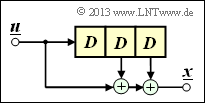
$\text{Example 3:}$ The impulse response of the shown third order digital filter is: $\underline{g} = (1, 0, 1, 1)$.
- Let the input sequence of this filter be unlimited in time: $\underline{u} = (1, 1, 0, 0, 0, \ \text{ ...})$.
- This gives the $($infinite$)$ initial sequence $\underline{x}$ in the binary Galois field ⇒ ${\rm GF(2)}$:
- \[\underline{x} = (\hspace{0.05cm}1,\hspace{0.05cm} 1,\hspace{0.05cm} 0,\hspace{0.05cm} 0,\hspace{0.05cm} 0, \hspace{0.05cm} \text{ ...} \hspace{0.05cm}) * (\hspace{0.05cm}1,\hspace{0.05cm} 0,\hspace{0.05cm} 1,\hspace{0.05cm} 1\hspace{0.05cm})\]
- \[\Rightarrow \hspace{0.3cm} \underline{x} =(\hspace{0.05cm}1,\hspace{0.05cm} 0,\hspace{0.05cm} 1,\hspace{0.05cm} 1,\hspace{0.05cm} 0, \hspace{0.05cm}0,\hspace{0.05cm} \text{ ...} \hspace{0.05cm}) \oplus (\hspace{0.05cm}0,\hspace{0.05cm}\hspace{0.05cm}1,\hspace{0.05cm} 0,\hspace{0.05cm} 1,\hspace{0.05cm} 1,\hspace{0.05cm}0, \hspace{0.05cm} \hspace{0.05cm} \text{ ...}\hspace{0.05cm}) = (\hspace{0.05cm}1,\hspace{0.05cm}\hspace{0.05cm}1,\hspace{0.05cm} 1,\hspace{0.05cm} 0,\hspace{0.05cm} 1,\hspace{0.05cm} 0, \hspace{0.05cm} \text{ ...} \hspace{0.05cm}) \hspace{0.05cm}.\]
- In the conventional convolution $($for real numbers$)$, on the other hand, the result would have been:
- \[\underline{x}= (\hspace{0.05cm}1,\hspace{0.05cm}\hspace{0.05cm}1,\hspace{0.05cm} 1,\hspace{0.05cm} 2,\hspace{0.05cm} 1,\hspace{0.05cm} 0, \text{ ...} \hspace{0.05cm}) \hspace{0.05cm}.\]
However, discrete time signals can also be represented by polynomials with respect to a dummy variable.
$\text{Definition:}$ The »D–transform« belonging to the discrete time signal $\underline{x} = (x_0, x_1, x_2, \ \text{...}) $ reads:
- \[X(D) = x_0 + x_1 \cdot D + x_2 \cdot D^2 + \hspace{0.05cm}\text{...}\hspace{0.05cm}= \sum_{i = 0}^{\infty} x_i \cdot D\hspace{0.05cm}^i \hspace{0.05cm}.\]
- For this particular transformation to an image area, we also use the following notation, where "D" stands for "delay operator":
- \[\underline{x} = (x_0, x_1, x_2,\hspace{0.05cm}...\hspace{0.05cm}) \quad \circ\!\!-\!\!\!-^{\hspace{-0.25cm}D}\!\!\!-\!\!\bullet\quad X(D) = \sum_{i = 0}^{\infty} x_i \cdot D\hspace{0.05cm}^i \hspace{0.05cm}.\]
Note: In the literature, sometimes $x(D)$ is used instead of $X(D)$. However, we write in our learning tutorial all image domain functions ⇒ "spectral domain functions" with capital letters, for example the Fourier transform, the Laplace transform and the D–transform:
- \[x(t) \hspace{0.15cm} \circ\!\!-\!\!\!-^{\hspace{-0.25cm}}\!\!\!-\!\!\bullet\hspace{0.15cm} X(f)\hspace{0.05cm},\hspace{0.4cm} x(t) \hspace{0.15cm} \circ\!\!-\!\!\!-^{\hspace{-0.25cm}\rm L}\!\!\!-\!\!\bullet\hspace{0.15cm} X(p) \hspace{0.05cm},\hspace{0.4cm} \underline{x} \hspace{0.15cm} \circ\!\!-\!\!\!-^{\hspace{-0.25cm}D}\!\!\!-\!\!\bullet\hspace{0.15cm} X(D) \hspace{0.05cm}.\]
We now apply the D–transform also
- to the information sequence $\underline{u}$, and
- the impulse response $\underline{g}$.
Due to the time limit of $\underline{g}$ the upper summation limit at $G(D)$ results in $i = m$:
- \[\underline{u} = (u_0, u_1, u_2,\hspace{0.05cm}\text{...}\hspace{0.05cm}) \quad \circ\!\!-\!\!\!-^{\hspace{-0.25cm}D}\!\!\!-\!\!\bullet\quad U(D) = \sum_{i = 0}^{\infty} u_i \cdot D\hspace{0.05cm}^i \hspace{0.05cm},\]
- \[\underline{g} = (g_0, g_1, \hspace{0.05cm}\text{...}\hspace{0.05cm}, g_m) \quad \circ\!\!-\!\!\!-^{\hspace{-0.25cm}D}\!\!\!-\!\!\bullet\quad G(D) = \sum_{i = 0}^{m} g_i \cdot D\hspace{0.05cm}^i \hspace{0.05cm}.\]
$\text{Theorem:}$ As with all spectral transformations, the »multiplication« applies to the D–transform in the image domain, since the $($discrete$)$ time functions $\underline{u}$ and $\underline{g}$ are interconnected by the »convolution«:
- \[\underline{x} = \underline{u} * \underline{g} \quad \circ\!\!-\!\!\!-^{\hspace{-0.25cm}D}\!\!\!-\!\!\bullet\quad X(D) = U(D) \cdot G(D) \hspace{0.05cm}.\]
- The $($rather simple$)$ $\rm proof$ of this important result can be found in the specification for "Exercise 3.3Z".
- As in »$\text{system theory}$« commonly, the D–transform $G(D)$ of the impulse response $\underline{g}$ is also called "transfer function".
$\text{Example 4:}$ We consider again the discrete time signals
- \[\underline{u} = (\hspace{0.05cm}1\hspace{0.05cm},\hspace{0.05cm} 1\hspace{0.05cm},\hspace{0.05cm} 0\hspace{0.05cm},\hspace{0.05cm} 0\hspace{0.05cm},\hspace{0.05cm}\text{...}\hspace{0.05cm}) \quad \circ\!\!-\!\!\!-^{\hspace{-0.25cm}D}\!\!\!-\!\!\bullet\quad U(D) = 1+ D \hspace{0.05cm},\]
- \[\underline{g} = (\hspace{0.05cm}1\hspace{0.05cm},\hspace{0.05cm} 0\hspace{0.05cm},\hspace{0.05cm} 1\hspace{0.05cm},\hspace{0.05cm} 1\hspace{0.05cm}) \quad \circ\!\!-\!\!\!-^{\hspace{-0.25cm}D}\!\!\!-\!\!\bullet\quad G(D) = 1+ D^2 + D^3 \hspace{0.05cm}.\]
- As in $\text{Example 3}$ $($in this section above$)$, you get also on this solution path:
- \[X(D) = U(D) \cdot G(D) = (1+D) \cdot (1+ D^2 + D^3) \]
- \[\Rightarrow \hspace{0.3cm} X(D) = 1+ D^2 + D^3 +D + D^3 + D^4 = 1+ D + D^2 + D^4 \hspace{0.3cm} \Rightarrow \hspace{0.3cm} \underline{x} = (\hspace{0.05cm}1\hspace{0.05cm},\hspace{0.05cm} 1\hspace{0.05cm},\hspace{0.05cm} 1\hspace{0.05cm},\hspace{0.05cm} 0\hspace{0.05cm},\hspace{0.05cm} 1\hspace{0.05cm},\hspace{0.05cm} 0\hspace{0.05cm}, \text{...} \hspace{0.05cm}) \hspace{0.05cm}.\]
- Multiplication by the "delay operator" $D$ in the image domain corresponds to a shift of one place to the right in the time domain:
- \[W(D) = D \cdot X(D) \quad \bullet\!\!-\!\!\!-^{\hspace{-0.25cm}D}\!\!\!-\!\!\circ\quad \underline{w} = (\hspace{0.05cm}0\hspace{0.05cm},\hspace{0.05cm}1\hspace{0.05cm},\hspace{0.05cm} 1\hspace{0.05cm},\hspace{0.05cm} 1\hspace{0.05cm},\hspace{0.05cm} 0\hspace{0.05cm},\hspace{0.05cm} 1\hspace{0.05cm},\hspace{0.05cm} 0\hspace{0.05cm}, \text{...} \hspace{0.05cm}) \hspace{0.05cm}.\]
Application of the D–transform to rate $1/n$ convolution encoders
We now apply the results of the last section to a convolutional encoder, restricting ourselves for the moment to the special case $k = 1$.
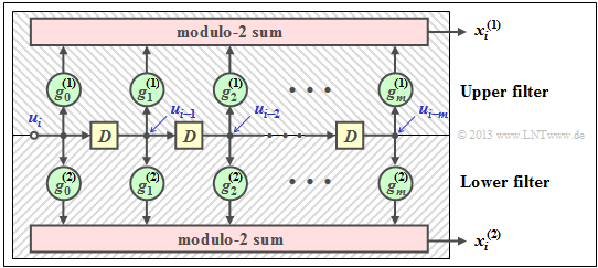
- Such a $(n, \ k = 1)$ convolutional code can be realized with $n$ digital filters operating in parallel on the same information sequence $\underline{u}$.
- The graph shows the arrangement for the code parameter $n = 2$ ⇒ code rate $R = 1/2$.
The following equations apply equally to both filters, setting $j = 1$ for the upper filter and $j = 2$ for the lower filter:
- The »impulse responses« of the two filters result in
- \[\underline{g}^{(j)} = (g_0^{(j)}, g_1^{(j)}, \hspace{0.05cm}\text{...}\hspace{0.05cm}, g_m^{(j)}\hspace{0.01cm}) \hspace{0.05cm},\hspace{0.2cm}{\rm with }\hspace{0.15cm} j \in \{1,2\}\hspace{0.05cm}.\]
- The two »output sequences« are as follows, considering that both filters operate on the same input sequence $\underline{u} = (u_0, u_1, u_2, \hspace{0.05cm} \text{...})$ :
- \[\underline{x}^{(j)} = (x_0^{(j)}, x_1^{(j)}, x_2^{(j)}, \hspace{0.05cm}\text{...}\hspace{0.05cm}) = \underline{u} \cdot \underline{g}^{(j)} \hspace{0.05cm},\hspace{0.2cm}{\rm with }\hspace{0.15cm} j \in \{1,2\}\hspace{0.05cm}.\]
- For the »D–transform« of the output sequences:
- \[X^{(j)}(D) = U(D) \cdot G^{(j)}(D) \hspace{0.05cm},\hspace{0.2cm}{\rm with }\hspace{0.15cm} j \in \{1,2\}\hspace{0.05cm}.\]
In order to represent this fact more compactly, we now define the following vectorial quantities of a convolutional code of rate $1/n$:
$\text{Definition:}$ The »D– transfer functions« of the $n$ parallel arranged digital filters are combined in the vector $\underline{G}(D)$:
- \[\underline{G}(D) = \left ( G^{(1)}(D), G^{(2)}(D), \hspace{0.05cm}\text{...}\hspace{0.1cm}, G^{(n)} (D) \right )\hspace{0.05cm}.\]
- The vector $\underline{X}(D)$ contains the D–transform of $n$ encoded sequences $\underline{x}^{(1)}, \underline{x}^{(2)}, \ \text{...} \ , \underline{x}^{(n)}$:
- \[\underline{X}(D) = \left ( X^{(1)}(D), X^{(2)}(D), \hspace{0.05cm}\text{...}\hspace{0.1cm}, X^{(n)} (D) \right )\hspace{0.05cm}.\]
- This gives the following vector equation:
- \[\underline{X}(D) = U(D) \cdot \underline{G}(D)\hspace{0.05cm}.\]
- $U(D)$ is not a vector quantity here because of the code parameter $k = 1$.
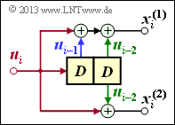
$\text{Example 5:}$ We consider the convolutional encoder with code parameters $n = 2, \ k = 1, \ m = 2$. For this one holds:
- \[\underline{g}^{(1)} =(\hspace{0.05cm}1\hspace{0.05cm},\hspace{0.05cm} 1\hspace{0.05cm},\hspace{0.05cm} 1\hspace{0.05cm}) \quad \circ\!\!-\!\!\!-^{\hspace{-0.25cm}D}\!\!\!-\!\!\bullet\quad G(D) = 1+ D + D^2 \hspace{0.05cm},\]
- \[\underline{g}^{(2)}= (\hspace{0.05cm}1\hspace{0.05cm},\hspace{0.05cm} 0\hspace{0.05cm},\hspace{0.05cm} 1\hspace{0.05cm}) \quad \circ\!\!-\!\!\!-^{\hspace{-0.25cm}D}\!\!\!-\!\!\bullet\quad G(D) = 1+ D^2 \]
- \[\Rightarrow \hspace{0.3cm} \underline{G}(D) = \big ( 1+ D + D^2 \hspace{0.05cm}, \hspace{0.1cm}1+ D^2 \big )\hspace{0.05cm}.\]
- Let the information sequence be $\underline{u} = (1, 0, 1, 1)$ ⇒ D–transform $U(D) = 1 + D^2 + D^3$. This gives:
- \[\underline{X}(D) = \left ( X^{(1)}(D),\hspace{0.1cm} X^{(2)}(D) \right ) = U(D) \cdot \underline{G}(D) \hspace{0.05cm}, \hspace{0.2cm}\]
- where
- \[{X}^{(1)}(D) = (1+ D^2 + D^3) \cdot (1+ D + D^2)=1+ D + D^2 + D^2 + D^3 + D^4 + D^3 + D^4 + D^5 = 1+ D + D^5\]
- \[\Rightarrow \hspace{0.3cm} \underline{x}^{(1)} = (\hspace{0.05cm}1\hspace{0.05cm},\hspace{0.05cm}1\hspace{0.05cm},\hspace{0.05cm} 0\hspace{0.05cm},\hspace{0.05cm} 0\hspace{0.05cm},\hspace{0.05cm} 0\hspace{0.05cm},\hspace{0.05cm} 1\hspace{0.05cm},\hspace{0.05cm} 0\hspace{0.05cm}, \hspace{0.05cm} 0\hspace{0.05cm}, \hspace{0.05cm} \text{...} \hspace{0.05cm} \hspace{0.05cm}) \hspace{0.05cm},\]
- \[{X}^{(2)}(D) = (1+ D^2 + D^3) \cdot (1+ D^2)=1+ D^2 + D^2 + D^4 + D^3 + D^5 = 1+ D^3 + D^4 + D^5\]
- \[\Rightarrow \underline{x}^{(2)} = (\hspace{0.05cm}1\hspace{0.05cm},\hspace{0.05cm}0\hspace{0.05cm},\hspace{0.05cm} 0\hspace{0.05cm},\hspace{0.05cm} 1\hspace{0.05cm},\hspace{0.05cm} 1\hspace{0.05cm},\hspace{0.05cm} 1\hspace{0.05cm},\hspace{0.05cm} 0\hspace{0.05cm}, \hspace{0.05cm} 0\hspace{0.05cm}, \hspace{0.05cm} \text{...} \hspace{0.05cm} \hspace{0.05cm}) \hspace{0.05cm}.\]
- We got the same result in "Exercise 3.1Z" on other way. After multiplexing the two strands, you get again:
- $$\underline{x} = (11, 10, 00, 01, 01, 11, 00, 00, \hspace{0.05cm} \text{...} \hspace{0.05cm}).$$
Transfer Function Matrix
We have seen that a convolutional code of rate $1/n$ can be most compactly described as a vector equation in the D–transformed domain:
- $$\underline{X}(D) = U(D) \cdot \underline{G}(D).$$
Now we extend the result to convolutional encoders with more than one input ⇒ $k ≥ 2$ $($see graph$)$.
In order to map a convolutional code of rate $k/n$ in the D–domain, the dimension of the above vector equation must be increased with respect to input and transfer function:
- \[\underline{X}(D) = \underline{U}(D) \cdot { \boldsymbol{\rm G}}(D)\hspace{0.05cm}.\]
This requires the following measures:
- From the scalar function $U(D)$ we get the vector
- $$\underline{U}(D) = (U^{(1)}(D), \ U^{(2)}(D), \hspace{0.05cm} \text{...} \hspace{0.05cm} , \ U^{(k)}(D)).$$
- From the vector $\underline{G}(D)$ we get the $k × n$ transfer function matrix $($or "polynomial generator matrix"$)$ $\mathbf{G}(D)$ :
- \[{\boldsymbol{\rm G}}(D)=\begin{pmatrix} G_1^{(1)}(D) & G_1^{(2)}(D) & \hspace{0.05cm} \text{...} \hspace{0.05cm} & G_1^{(n)}(D)\\ G_2^{(1)}(D) & G_2^{(2)}(D) & \hspace{0.05cm} \text{...} \hspace{0.05cm} & G_2^{(n)}(D)\\ \vdots & \vdots & & \vdots\\ G_k^{(1)}(D) & G_k^{(2)}(D) & \hspace{0.05cm} \text{...} \hspace{0.05cm} & G_k^{(n)}(D) \end{pmatrix}\hspace{0.05cm}.\]
- Each of the $k \cdot n$ matrix elements $G_i^{(j)}(D)$ with $1 ≤ i ≤ k,\ 1 ≤ j ≤ n$ is a polynomial over the dummy variable $D$ in the Galois field ${\rm GF}(2)$, maximal of degree $m$, where $m$ denotes the memory.
- For the above transfer function matrix, using the »$\text{partial matrices}$« $\mathbf{G}_0, \ \text{...} \ , \mathbf{G}_m$ also be written $($as index we use again $l)$:
- \[{\boldsymbol{\rm G}}(D) = \sum_{l = 0}^{m} {\boldsymbol{\rm G}}_l \cdot D\hspace{0.03cm}^l = {\boldsymbol{\rm G}}_0 + {\boldsymbol{\rm G}}_1 \cdot D + {\boldsymbol{\rm G}}_2 \cdot D^2 + \hspace{0.05cm} \text{...} \hspace{0.05cm}+ {\boldsymbol{\rm G}}_m \cdot D\hspace{0.03cm}^m \hspace{0.05cm}.\]
$\text{Example 6:}$ We consider the $(n = 3, \ k = 2, \ m = 1)$ convolutional encoder whose partial matrices have already been determined in the $\text{Example 1}$ as follows:
- \[{ \boldsymbol{\rm G} }_0 = \begin{pmatrix} 1 & 0 & 1\\ 0 & 1 & 1 \end{pmatrix} \hspace{0.05cm}, \hspace{0.5cm} { \boldsymbol{\rm G} }_1 = \begin{pmatrix} 1 & 1 & 1\\ 1 & 0 & 0 \end{pmatrix}\hspace{0.05cm}.\]
- Because of $m = 1$ no partial matrices exist for $l ≥ 2$. Thus the transfer function matrix is:
- \[{\boldsymbol{\rm G} }(D) = {\boldsymbol{\rm G} }_0 + {\boldsymbol{\rm G} }_1 \cdot D = \begin{pmatrix} 1+D & D & 1+D\\ D & 1 & 1 \end{pmatrix} \hspace{0.05cm}.\]
- Let the $($time limited$)$ information sequence be $\underline{u} = (0, 1, 1, 0, 0, 0, 1, 1)$, from which the two input sequences are as follows:
- \[\underline{u}^{(1)} = (\hspace{0.05cm}0\hspace{0.05cm},\hspace{0.05cm}1\hspace{0.05cm},\hspace{0.05cm} 0\hspace{0.05cm},\hspace{0.05cm} 1\hspace{0.05cm}) \quad \circ\!\!-\!\!\!-^{\hspace{-0.25cm}D}\!\!\!-\!\!\bullet\quad {U}^{(1)}(D) = D + D^3 \hspace{0.05cm},\]
- \[\underline{u}^{(2)} = (\hspace{0.05cm}1\hspace{0.05cm},\hspace{0.05cm}0\hspace{0.05cm},\hspace{0.05cm} 0\hspace{0.05cm},\hspace{0.05cm} 1\hspace{0.05cm}) \quad \circ\!\!-\!\!\!-^{\hspace{-0.25cm}D}\!\!\!-\!\!\bullet\quad {U}^{(2)}(D) = 1 + D^3 \hspace{0.05cm}.\]
- From this follows for the vector of the D–transform at the encoder output:
- \[\underline{X}(D) = \big (\hspace{0.05cm} {X}^{(1)}(D)\hspace{0.05cm}, \hspace{0.05cm} {X}^{(2)}(D)\hspace{0.05cm}, \hspace{0.05cm} {X}^{(3)}(D)\hspace{0.05cm}\big ) = \underline{U}(D) \cdot {\boldsymbol{\rm G} }(D) \begin{pmatrix} D+D^3 & 1+D^3 \end{pmatrix} \cdot \begin{pmatrix} 1+D & D & 1+D\\ D & 1 & 1 \end{pmatrix}\hspace{0.05cm}.\]
- This results in the following encoded sequences in the three strands:
- \[{X}^{(1)}(D) = (D + D^3) \cdot (1+D) + (1 + D^3) \cdot D =D + D^2 + D^3 + D^4 + D + D^4 = D^2 + D^3\]
- \[\Rightarrow \hspace{0.3cm} \underline{x}^{(1)} = (\hspace{0.05cm}0\hspace{0.05cm},\hspace{0.05cm}0\hspace{0.05cm},\hspace{0.05cm} 1\hspace{0.05cm},\hspace{0.05cm} 1\hspace{0.05cm},\hspace{0.05cm}\hspace{0.05cm} 0\hspace{0.05cm},\hspace{0.05cm}\hspace{0.05cm} 0\hspace{0.05cm},\hspace{0.05cm} \text{...} \hspace{0.05cm}) \hspace{0.05cm},\]
- \[{X}^{(2)}(D)= (D + D^3) \cdot D + (1 + D^3) \cdot 1 = D^2 + D^4 + 1 + D^3 = 1+D^2 + D^3 + D^4\]
- \[\Rightarrow \hspace{0.3cm}\underline{x}^{(2)} = (\hspace{0.05cm}1\hspace{0.05cm},\hspace{0.05cm}0\hspace{0.05cm},\hspace{0.05cm} 1\hspace{0.05cm},\hspace{0.05cm} 1\hspace{0.05cm},\hspace{0.05cm} 1\hspace{0.05cm},\hspace{0.05cm}\hspace{0.05cm} 0\hspace{0.05cm},\hspace{0.05cm}\hspace{0.05cm} \text{...} \hspace{0.05cm}) \hspace{0.05cm},\]
- \[{X}^{(3)}(D)=(D + D^3) \cdot (1 + D) + (1 + D^3) \cdot 1 = D + D^2 + D^3+ D^4 + 1 + D^3 = 1+ D + D^2 + D^4\]
- \[\Rightarrow \hspace{0.3cm}\underline{x}^{(3)} = (\hspace{0.05cm}1\hspace{0.05cm},\hspace{0.05cm}1\hspace{0.05cm},\hspace{0.05cm} 1\hspace{0.05cm},\hspace{0.05cm} 0\hspace{0.05cm},\hspace{0.05cm} 1\hspace{0.05cm},\hspace{0.05cm}\hspace{0.05cm} 0\hspace{0.05cm},\hspace{0.05cm}\hspace{0.05cm} \text{...} \hspace{0.05cm}) \hspace{0.05cm}.\]
We have already obtained the same results in other ways in previous examples:
- in $\text{Example 4}$ of the chapter "Basics of Convolutional Coding",
- in $\text{Example 2}$ of the current chapter.
Systematic convolutional codes
Polynomial representation using the transfer function matrix $\mathbf{G}(D)$ provides insight into the structure of a convolutional code.
- This $k × n$ matrix is used to recognize whether it is a »$\text{systematic code}$«.
- This refers to a code where the encoded sequences $\underline{x}^{(1)}, \ \text{...} \ , \ \underline{x}^{(k)}$ are identical with the information sequences $\underline{u}^{(1)}, \ \text{...} \ , \ \underline{u}^{(k)}$.
- The graph shows an example of a systematic $(n = 4, \ k = 3)$ convolutional code.
A systematic $(n, k)$ convolutional code exists whenever the transfer function matrix $($with $k$ rows and $n$ columns$)$ has the following appearance:
- \[{\boldsymbol{\rm G}}(D) = {\boldsymbol{\rm G}}_{\rm sys}(D) = \left [ \hspace{0.05cm} {\boldsymbol{\rm I}}_k\hspace{0.05cm} ; \hspace{0.1cm} {\boldsymbol{\rm P}}(D) \hspace{0.05cm}\right ] \hspace{0.05cm}.\]
The following nomenclature is used:
- $\mathbf{I}_k$ denotes a diagonal unit matrix of dimension $k × k$.
- $\mathbf{P}(D)$ is a $k × (n -k)$ matrix, where each matrix element describes a polynomial in $D$.
$\text{Example 7:}$ A systematic convolutional code with $n = 3, \ k = 2, \ m = 2$ might have the following transfer function matrix:
- \[{\boldsymbol{\rm G} }_{\rm sys}(D) = \begin{pmatrix} 1 & 0 & 1+D^2\\ 0 & 1 & 1+D \end{pmatrix}\hspace{0.05cm}.\]
- In contrast, other systematic convolutional codes with equal $n$ and equal $k$ differ only by the two matrix elements in the last column.
Equivalent systematic convolutional code
For every $(n, \ k)$ convolutional code with matrix $\mathbf{G}(D)$ there is an "equivalent systematic code" whose D–matrix we denote by $\mathbf{G}_{\rm sys}(D)$.
To get from the transfer function matrix $\mathbf{G}(D)$ to the matrix $\mathbf{G}_{\rm sys}(D)$ of the equivalent systematic convolutional code, proceed as follows according to the diagram:
- Divide the $k × n$ matrix $\mathbf{G}(D)$ into a square matrix $\mathbf{T}(D)$ with $k$ rows and $k$ columns and denote the remainder by $\mathbf{Q}(D)$.
- Then calculate the inverse matrix $\mathbf{T}^{-1}(D)$ to $\mathbf{T}(D)$ and from this the matrix for the equivalent systematic code:
- \[{\boldsymbol{\rm G}}_{\rm sys}(D)= {\boldsymbol{\rm T}}^{-1}(D) \cdot {\boldsymbol{\rm G}}(D) \hspace{0.05cm}.\]
- Since the product $\mathbf{T}^{-1}(D) \cdot \mathbf{T}(D)$ yields the $k × k$ unit matrix $\mathbf{I}_k$
⇒ the transfer function matrix of the equivalent systematic code can be written in the desired form:
- \[{\boldsymbol{\rm G}}_{\rm sys}(D) = \bigg [ \hspace{0.05cm} {\boldsymbol{\rm I}}_k\hspace{0.05cm} ; \hspace{0.1cm} {\boldsymbol{\rm P}}(D) \hspace{0.05cm}\bigg ] \hspace{0.5cm}{\rm with}\hspace{0.5cm} {\boldsymbol{\rm P}}(D)= {\boldsymbol{\rm T}}^{-1}(D) \cdot {\boldsymbol{\rm Q}}(D) \hspace{0.05cm}. \hspace{0.05cm}\]
$\text{Example 8:}$
The encoder of rate $2/3$ considered often in the last sections is not systematic because e.g. $\underline{x}^{(1)} ≠ \underline{u}^{(1)}, \ \underline{x}^{(2)} ≠ \underline{u}^{(2)}$ holds $($see adjacent graphic$)$.
⇒ However, this can also be seen from the transfer function matrix:
- \[{\boldsymbol{\rm G} }(D) = \big [ \hspace{0.05cm} {\boldsymbol{\rm T} }(D)\hspace{0.05cm} ; \hspace{0.1cm} {\boldsymbol{\rm Q} }(D) \hspace{0.05cm}\big ]\]
- \[\Rightarrow \hspace{0.3cm} {\boldsymbol{\rm T} }(D) = \begin{pmatrix} 1+D & D\\ D & 1 \end{pmatrix}\hspace{0.05cm},\hspace{0.2cm} {\boldsymbol{\rm Q} }(D) = \begin{pmatrix} 1+D \\ 1 \end{pmatrix}\hspace{0.05cm}.\]
- The determinant of $\mathbf{T}(D)$ results in $(1 + D) \cdot 1 + D \cdot D = 1 + D + D^2$ and is nonzero.
- Thus, for the inverse of $\mathbf{T}(D)$ can be written $($swapping the diagonal elements!$)$:
- \[{\boldsymbol{\rm T} }^{-1}(D) = \frac{1}{1+D+D^2} \cdot \begin{pmatrix} 1 & D\\ D & 1+D \end{pmatrix}\hspace{0.05cm}.\]
- The product $\mathbf{T}(D) \cdot \mathbf{T}^{–1}(D)$ gives the unit matrix $\mathbf{I}_2$ ⇒ for the third column of $\mathbf{G}_{\rm sys}(D)$ holds:
- \[{\boldsymbol{\rm P} }(D)= {\boldsymbol{\rm T} }^{-1}(D) \cdot {\boldsymbol{\rm Q} }(D) = \frac{1}{1+D+D^2} \cdot \begin{pmatrix} 1 & D\\ D & 1+D \end{pmatrix}\cdot \begin{pmatrix} 1+D\\ 1 \end{pmatrix} \]
- \[\Rightarrow \hspace{0.3cm} {\boldsymbol{\rm P} }(D) = \frac{1}{1+D+D^2} \cdot \begin{pmatrix} (1+D) + D \\ D \cdot (1+D) + (1+D) \end{pmatrix} = \frac{1}{1+D+D^2} \cdot \begin{pmatrix} 1 \\ 1+D^2 \end{pmatrix} \]
- \[\Rightarrow \hspace{0.2cm}{\boldsymbol{\rm G} }_{\rm sys}(D) = \begin{pmatrix} 1 & 0 & \frac{1}{1+D+D^2}\\ 0 & 1 &\frac{1+D^2}{1+D+D^2} \end{pmatrix}\hspace{0.05cm}. \]
It remains to be clarified what the filter of such a fractional–rational transfer function looks like.
Filter structure with fractional–rational transfer function
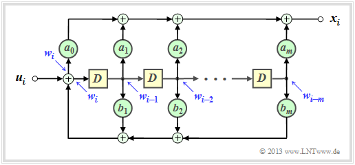
If a transfer function has the form $G(D) = A(D)/B(D)$, the associated filter is called »recursive«. Given a recursive convolutional encoder with memory $m$, the two polynomials $A(D)$ and $B(D)$ can be written in general terms:
- \[A(D) = \sum_{l = 0}^{m} a_l \cdot D\hspace{0.05cm}^l = a_0 + a_1 \cdot D + a_2 \cdot D^2 +\ \text{...} \ \hspace{0.05cm} + a_m \cdot D\hspace{0.05cm}^m \hspace{0.05cm},\]
- \[B(D) = 1 + \sum_{l = 1}^{m} b_l \cdot D\hspace{0.05cm}^l = 1 + b_1 \cdot D + b_2 \cdot D^2 + \ \text{...} \ \hspace{0.05cm} + b_m \cdot D\hspace{0.05cm}^m \hspace{0.05cm}.\]
The graphic shows the corresponding filter structure in the so–called "Controller Canonical Form":
- The coefficients $a_0, \ \text{...} \ , \ a_m$ describe the forward branch.
- The coefficients $b_1, \ \text{...} \ , \ b_m$ form a feedback branch.
- All coefficients are binary,
- so $1$ $($continuous connection$)$
- or $0$ $($missing connection$)$.
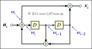
$\text{Example 9:}$ The filter structure outlined on the right can be described as follows:
- \[x_i = w_i + w_{i-2} \hspace{0.05cm},\]
- \[w_i = u_i + w_{i-1}+ w_{i-2} \hspace{0.05cm}.\]
- Accordingly, for the D–transforms:
- \[X(D) =W(D) + W(D) \cdot D^2 =W(D) \cdot \left ( 1+ D^2 \right ) \hspace{0.05cm},\]
- \[W(D) = \hspace{0.08cm} U(D) + W(D) \cdot D+ W(D) \cdot D^2\]
- \[\Rightarrow \hspace{0.3cm} U(D) = W(D) \cdot \left ( 1+ D + D^2 \right ) \hspace{0.05cm}.\]
- Thus, one obtains for the transfer function of this filter:
- \[G(D) = \frac{X(D)}{U(D)} = \frac{1+D^2}{1+D+D^2} \hspace{0.05cm}. \]
- In $\text{Example 8}$ to the equivalent systematic convolutional code, exactly this expression has resulted in the lower branch.
Exercises for the chapter
Exercise 3.2: G-matrix of a Convolutional Encoder
Exercise 3.2Z: (3, 1, 3) Convolutional Encoder
Exercise 3.3: Code Sequence Calculation via U(D) and G(D)
Exercise 3.3Z: Convolution and D-Transformation
Exercise 3.4: Systematic Convolution Codes
Exercise 3.4Z: Equivalent Convolution Codes?
Exercise 3.5: Recursive Filters for GF(2)
