Difference between revisions of "Channel Coding/The Basics of Turbo Codes"
| (51 intermediate revisions by 6 users not shown) | |||
| Line 1: | Line 1: | ||
{{Header | {{Header | ||
| − | |Untermenü=Iterative | + | |Untermenü=Iterative Decoding Methods |
| − | |Vorherige Seite= | + | |Vorherige Seite=The Basics of Product Codes |
| − | |Nächste Seite= | + | |Nächste Seite=The Basics of Low-Density Parity Check Codes |
}} | }} | ||
| − | == | + | == Basic structure of a turbo code == |
<br> | <br> | ||
| − | + | All communications systems current today $($2017$)$, such as | |
| + | * [[Examples_of_Communication_Systems/General_Description_of_UMTS#.23_OVERVIEW_OF_THE_FOURTH_MAIN_CHAPTER_.23|$\rm UMTS$]] $($"Universal Mobile Telecommunications System" ⇒ 3rd generation mobile communications$)$ and | ||
| + | *[[Mobile_Communications/General_Information_on_the_LTE_Mobile_Communications_Standard#.23_OVERVIEW_OF_THE_FOURTH_MAIN_CHAPTER_.23|$\rm LTE$]] $($"Long Term Evolution" ⇒ 4th generation mobile communications$)$ | ||
| − | |||
| − | [[ | + | use the concept of [[Channel_Coding/Soft-in_Soft-Out_Decoder#Bit-wise_soft-in_soft-out_decoding|$\text{symbol-wise iterative decoding}$]]. This is directly related to the invention of »'''turbo codes'''« in 1993 by [https://en.wikipedia.org/wiki/Claude_Berrou $\text{Claude Berrou}$], [https://en.wikipedia.org/wiki/Alain_Glavieux $\text{Alain Glavieux}$] and [https://scholar.google.com/citations?user=-UZolIAAAAAJ $\text{Punya Thitimajshima}$] because it was only with these codes that the Shannon bound could be approached with reasonable decoding effort.<br> |
| − | + | Turbo codes result from the parallel or serial concatenation of convolutional codes. | |
| − | + | [[File:EN_KC_T_4_3_S1a_v1.png|right|frame|Parallel concatenation of two rate $1/2$ codes|class=fit]] | |
| + | [[File:EN_KC_T_4_3_S1b_v1.png|right|frame|Rate $1/3$ turbo encoder $($parallel concatenation of two rate $1/2$ convolutional codes$)$ |class=fit]] | ||
| + | The graphic shows the parallel concatenation of two codes, each with the parameters $k = 1, \ n = 2$ ⇒ code rate $R = 1/2$.<br> | ||
| − | + | In this representation is: | |
| + | # $u$ the currently considered bit of the information sequence $\underline{u}$,<br> | ||
| + | # $x_{i,\hspace{0.03cm}j}$ the currently considered bit at the output $j$ of encoder $i$ <br>$($with $1 ≤ i ≤ 2, \hspace{0.2cm} 1 ≤ j ≤ 2)$,<br> | ||
| + | # $\underline{X} = (x_{1,\hspace{0.03cm}1}, \ x_{1,\hspace{0.03cm}2}, \ x_{2,\hspace{0.03cm}1}, \ x_{2,\hspace{0.03cm}2})$ the code word for the current information bit $u$.<br><br> | ||
| − | + | The resulting rate of the concatenated coding system is thus $R = 1/4$. | |
| − | + | If systematic component codes are used, the second shown model results. The modifications from the top graph to the graph below can be justified as follows: | |
| + | *For systematic codes $C_1$ and $C_2$, both $x_{1,\hspace{0.03cm}1} = u$ and $x_{2,\hspace{0.03cm}1} = u$. Therefore, one can dispense with the transmission of a redundant bit $($e.g. $x_{2,\hspace{0.03cm}2})$. | ||
| − | + | *With this reduction, the result is a rate $1/3$ turbo code with $k = 1$ and $n = 3$. The code word with the parity bits is $p_1$ $($encoder 1$)$ and $p_2$ $($encoder 2$)$: | |
| + | :$$\underline{X} = \left (u, \ p_1, \ p_2 \right )\hspace{0.05cm}.$$ | ||
| − | |||
| − | + | == Further modification of the basic structure of the turbo code== | |
| − | + | <br> | |
| + | In the following we always assume a still somewhat further modified turbo encoder model: | ||
| + | [[File:EN_KC_T_4_3_S1c_v2.png|right|frame|Rate $1/3$ turbo encoder with interleaver|class=fit]] | ||
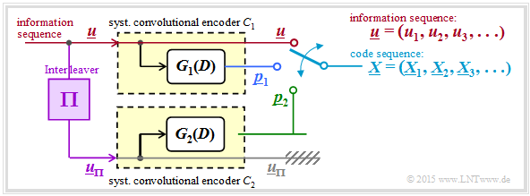
| − | + | #As required for the description of convolutional codes, at the input is the information sequence $\underline{u} = (u_1, \ u_2, \ \text{...}\hspace{0.05cm} , \ u_i , \ \text{...}\hspace{0.05cm} )$ instead of the isolated information bit $u$ .<br> | |
| + | #The code word sequence $\underline{x} = (\underline{X}_1, \underline{X}_2, \ \text{...}\hspace{0.05cm} , \ \underline{X}_i, \ \text{...}\hspace{0.05cm} )$ is generated. To avoid confusion, the code words $\underline{X}_i = (u, \ p_1, \ p_2)$ with capital letters were introduced in the last section.<br> | ||
| + | #The encoders $\mathcal{C}_1$ and $\mathcal{C}_2$ are conceived $($at least in thought$)$ as [[Theory_of_Stochastic_Signals/Digital_Filters| $\text{digital filters}$]] and are thus characterized by the [[Channel_Coding/Algebraic_and_Polynomial_Description#Application_of_the_D.E2.80.93transform_to_rate_.7F.27.22.60UNIQ-MathJax158-QINU.60.22.27.7F_convolution_encoders| $\text{transfer functions}$]] $G_1(D)$ and $G_2(D)$.<br> | ||
| + | #For various reasons ⇒ see [[Channel_Coding/The_Basics_of_Turbo_Codes#Second_requirement_for_turbo_codes:_Interleaving| "two sections ahead"]] the input sequence of the second encoder ⇒ $\underline{u}_{\pi}$ should be scrambled with respect to the sequence $\underline{u}$ by an interleaver $(\Pi)$.<br> | ||
| + | #Thereby there is nothing against choosing both encoders the same: $G_1(D) = G_2(D) = G(D)$. Without interleaver the correction capability would be extremely limited.<br><br> | ||
| + | {{GraueBox|TEXT= | ||
| + | [[File:EN_KC_T_4_3_S1d_v2.png|right|frame|Example sequences at the rate $1/3$ turbo encoder|class=fit]] | ||
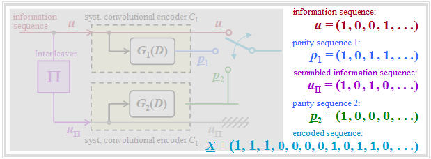
| + | $\text{Example 1:}$ The graph shows the different sequences in matched colors. To note: | ||
| + | #For $\underline{u}_{\Pi}$ a $3×4$ interleaver matrix is considered according to [[Aufgaben:Exercise_4.08Z:_Basics_about_Interleaving|"Exercise 4.8Z"]].<br><br> | ||
| + | #The parity sequences are obtained according to $G_1(D) = G_2(D) = 1 + D^2$ ⇒ see [[Aufgaben:Exercise_4.08:_Repetition_to_the_Convolutional_Codes|"Exercise 4.8"]].}}<br> | ||
| − | == | + | == First requirement for turbo codes: Recursive component codes == |
<br> | <br> | ||
| − | + | Non-recursive transfer functions for generating the parity sequences cause a turbo code with insufficiently small minimum distance. The reason for this inadequacy is the finite impulse response $\underline{g} = (1, \ g_2, \ \text{...}\hspace{0.05cm} , \ g_m, \ 0, \ 0, \ \text{...}\hspace{0.05cm} )$ with $g_2, \ \text{...}\hspace{0.05cm} , \ g_m ∈ \{0, 1\}$. Here $m$ denotes the "memory".<br> | |
| − | + | [[File:EN_KC_T_4_3_S2a_v1.png|right|frame|Non-recursive systematic turbo code and state transition diagram|class=fit]] | |
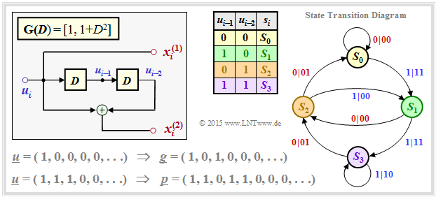
| − | + | <br><br>The graph shows the state transition diagram for the example $\mathbf{G}(D) = \big [1, \ 1 + D^2 \big ]$. The transitions are labeled "$u_i\hspace{0.05cm}|\hspace{0.05cm}u_i p_i$". | |
| + | *The sequence $S_0 → S_1 → S_2 → S_0 → S_0 → \ \text{...}\hspace{0.05cm} \ $ leads with respect to the input to the information sequence $\underline{u} = (1, 0, 0, 0, 0, \ \text{...}\hspace{0.05cm})$, and | ||
| − | [[File: | + | *with respect to the second encoded symbol to the sequence $\underline{p} = (1, 0, 1, 0, 0, \ \text{...}\hspace{0.05cm})$ ⇒ because of $\underline{u} = (1, 0, 0, 0, 0, \ \text{...}\hspace{0.05cm})$ identical to the "impulse response" $\underline{g}$ ⇒ memory $m = 2$.<br> |
| − | + | <br clear=all> | |
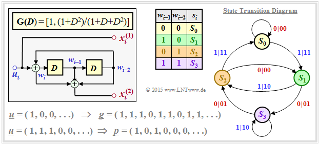
| − | + | The lower graph applies to a so-called »'''RSC code'''« $($"Recursive Systematic Convolutional"$)$ correspondingly | |
| − | + | [[File:EN_KC_T_4_3_S2b_v1.png|right|frame|Non-recursive systematic turbo code and state transition diagram|class=fit]] | |
| − | * | + | :$$\mathbf{G}(D) = \big [1, \ (1+ D^2)/(1 + D + D^2)\big ].$$ |
| + | *Here the sequence | ||
| + | :$$S_0 → S_1 → S_3 → S_2 → S_1 → S_3 → S_2 → \text{...}$$ | ||
| + | :leads to the impulse response | ||
| + | :$$\underline{g} = (1, 1, 1, 0, 1, 1, 0, 1, 1, \ \text{...}\hspace{0.05cm}).$$ | ||
| + | *This impulse response continues to infinity due to the loop $S_1 → S_3 → S_2 → S_1$. This enables or facilitates the iterative decoding.<br> | ||
| − | |||
| − | + | More details on the examples in this section can be found in the [[Aufgaben:Exercise_4.08Z:_Basics_about_Interleaving|"Exercise 4.8"]] and the [[Aufgaben:Exercise_4.09:_Recursive_Systematic_Convolutional_Codes|"Exercise 4.9"]].<br> | |
| − | |||
| − | |||
| − | |||
| − | + | == Second requirement for turbo codes: Interleaving == | |
| − | |||
| − | == | ||
<br> | <br> | ||
| − | + | It is obvious that for $G_1(D) = G_2(D)$ an interleaver $(\Pi)$ is essential. | |
| + | *Another reason is that the a-priori information is assumed to be independent. | ||
| − | + | *Thus, adjacent $($and thus possibly strongly dependent$)$ bits for the other sub–code should be far apart.<br> | |
| − | |||
| − | + | Indeed, for any RSC code ⇒ infinite impulse response $\underline{g}$ ⇒ fractional–rational transfer function $G(D)$: There are certain input sequences $\underline{u}$, which lead to very short parity sequences $\underline{p} = \underline{u} ∗ \underline{g}$ with low Hamming weight $w_{\rm H}(\underline{p})$. | |
| − | [[ | + | For example, such a sequence is given in the second graphic of the [[Channel_Coding/The_Basics_of_Turbo_Codes#First_requirement_for_turbo_codes:_Recursive_component_codes| "last section"]] : |
| + | :$$\underline{u} = (1, 1, 1, 0, 0, \ \text{...}\hspace{0.05cm}).$$ | ||
| + | Then for the output sequence holds: | ||
| − | + | ::<math>P(D) = U(D) \cdot G(D) = (1+D+D^2) \cdot \frac{1+D^2}{1+D+D^2}= 1+D^2\hspace{0.3cm}\Rightarrow\hspace{0.3cm} \underline{p}= (\hspace{0.05cm}1\hspace{0.05cm},\hspace{0.05cm} 0\hspace{0.05cm},\hspace{0.05cm} 1\hspace{0.05cm},\hspace{0.05cm} 0\hspace{0.05cm},\hspace{0.05cm} 0\hspace{0.05cm},\hspace{0.05cm} \text{...}\hspace{0.05cm}\hspace{0.05cm})\hspace{0.05cm}. </math> | |
| − | = | + | {{BlaueBox|TEXT= |
| − | + | $\text{Meaning and purpose:}$ | |
| − | + | By $\rm interleaving$, it is now ensured with high probability that this sequence $\underline{u} = (1, 1, 1, 0, 0, \ \text{...}\hspace{0.05cm})$ is converted into a sequence $\underline{u}_{\pi}$ | |
| + | *which also contains only three "ones",<br> | ||
| − | + | *but whose output sequence is characterized by a large Hamming weight $w_{\rm H}(\underline{p})$.<br> | |
| − | |||
| − | + | Thus, the decoder succeeds in resolving such "problem sequences" iteratively.}}<br> | |
| − | {{ | + | For the following description of the interleavers we use the assignment $I_{\rm In} → I_{\rm Out}$. These labels stand for the indices of output and input sequence, respectively. The interleaver variable is named $I_{\rm max}$ .<br> |
| − | + | [[File:P ID3048 KC T 4 3 S3a v5.png|right|frame|Clarification of block interleaving]] | |
| − | |||
| − | |||
| − | + | There are several, fundamentally different interleaver concepts:<br> | |
| − | + | ⇒ In a »<b>block interleaver</b>« one fills a matrix with $N_{\rm C}$ columns and $N_{\rm R}$ rows column-by-column and reads the matrix row-by-row. Thus an information block with $I_{\rm max} = N_{\rm C} \cdot N_{\rm R}$ bit is deterministically scrambled.<br> | |
| − | + | The right graph illustrates the principle for $I_{\rm max} = 64$ ⇒ $1 ≤ I_{\rm In} \le 64$ and $1 ≤ I_{\rm Out} \le 64$. The order of the output bits is then: | |
| − | + | :$$1, 9, 17, 25, 33, 41, 49, 57, 2, 10, 18, \ \text{...}\hspace{0.05cm} , 48, 56, 64.$$ | |
| − | + | More information on block interleaving is available in the [[Aufgaben:Exercise_4.08Z:_Basics_about_Interleaving|"Exercise 4.8Z"]].<br> | |
| − | + | [[File:P ID3050 KC T 4 3 S3b v5.png|left|frame|Clarification of $S$–random interleaving]] | |
| + | <br><br><br><br> | ||
| + | ⇒ Turbo codes often use the »'''$S$–random interleaver'''«. This pseudo random algorithm with the parameter "$S$" guarantees | ||
| + | *that two indices less than $S$ apart at the input | ||
| − | + | *occur at least at the distance $S + 1$ at the output. | |
| − | |||
| − | + | The left graph shows the $S$–random characteristic $I_{\rm Out}(I_{\rm In})$ for $I_{\rm max} = 640$.<br> | |
| − | |||
| − | + | #This algorithm is also deterministic, and one can undo the scrambling in the decoder ⇒ "De–interleaving". | |
| + | #The distribution still seems "more random" than with block interleaving. | ||
<br clear=all> | <br clear=all> | ||
| − | == | + | == Bit-wise iterative decoding of a turbo code == |
<br> | <br> | ||
| − | + | The decoding of a turbo code is basically done as described in section [[Channel_Coding/Soft-in_Soft-Out_Decoder#Bit-wise_soft-in_soft-out_decoding|"Bit-wise Soft–in Soft–out Decoding"]]. From the following graphic, however, you can also see some special features that apply only to the turbo decoder.<br> | |
| − | [[File: | + | Assumed is a rate $1/3$ turbo code according to the description in the [[Channel_Coding/The_Basics_of_Turbo_Codes#Basic_structure_of_a_turbo_code| "first section of this page"]]. Also, the color scheme for the information sequence $\underline{u}$ and the two parity sequences $\underline{p}_1$ and $\underline{p}_2$ are adapted from the earlier graphics. Further, it should be noted: |
| + | [[File:EN_KC_T_4_3_S4a_v2.png|right|frame|Iterative turbo decoder for rate $R = 1/3$ |class=fit]] | ||
| − | + | *The received vectors $\underline{y}_0,\hspace{0.15cm} \underline{y}_1,\hspace{0.15cm} \underline{y}_2$ are real-valued and provide the respective soft information with respect to the information sequence $\underline{u}$ and the sequences $\underline{p}_1$ $($parity for encoder 1$)$ and $\underline{p}_2$ $($parity for encoder 2$)$.<br> | |
| − | |||
| − | * | + | *The decoder 1 receives the required intrinsic information in the form of the $L$ values $L_{\rm K,\hspace{0.03cm} 0}$ $($out $\underline{y}_0)$ and $L_{\rm K,\hspace{0.03cm}1}$ $($out $\underline{y}_1)$ over each bit of the sequences $\underline{u}$ and $\underline{p}_1$. |
| − | * | + | *In the second decoder, the scrambling of the information sequence $\underline{u}$ must be taken into account. Thus, the $L$ values to be processed are $\pi(L_{\rm K, \hspace{0.03cm}0})$ and $L_{\rm K, \hspace{0.03cm}2}$.<br> |
| − | * | + | *In the general [[Channel_Coding/Soft-in_Soft-Out_Decoder#Basic_structure_of_concatenated_coding_systems|$\text{SISO decoder}$]] the information exchange between the two component decoders was controlled with $\underline{L}_{\rm A, \hspace{0.03cm}2} = \underline{L}_{\rm E, \hspace{0.03cm}1}$ and $\underline{L}_{\rm A, \hspace{0.03cm}1} = \underline{L}_{\rm E, \hspace{0.03cm}2}$. |
| + | |||
| + | *Written out at the bit level, these equations are denoted by $(1 ≤ i ≤ n)$: | ||
::<math>L_{\rm A, \hspace{0.03cm}2}(i) = L_{\rm E, \hspace{0.03cm}1}(i) | ::<math>L_{\rm A, \hspace{0.03cm}2}(i) = L_{\rm E, \hspace{0.03cm}1}(i) | ||
| − | \hspace{0.5cm}{\rm | + | \hspace{0.5cm}{\rm resp.}\hspace{0.5cm} |
L_{\rm A, \hspace{0.03cm}1}(i) = L_{\rm E, \hspace{0.03cm}2}(i) \hspace{0.03cm}.</math> | L_{\rm A, \hspace{0.03cm}1}(i) = L_{\rm E, \hspace{0.03cm}2}(i) \hspace{0.03cm}.</math> | ||
| − | * | + | *In the case of the turbo decoder, the interleaver must also be taken into account in this information exchange. Then for $i = 1, \ \text{...}\hspace{0.05cm} , \ n$: |
::<math>L_{\rm A, \hspace{0.03cm}2}\left ({\rm \pi}(i) \right ) = L_{\rm E, \hspace{0.03cm}1}(i) | ::<math>L_{\rm A, \hspace{0.03cm}2}\left ({\rm \pi}(i) \right ) = L_{\rm E, \hspace{0.03cm}1}(i) | ||
| Line 130: | Line 152: | ||
L_{\rm A, \hspace{0.03cm}1}(i) = L_{\rm E, \hspace{0.03cm}2}\left ({\rm \pi}(i) \right ) \hspace{0.05cm}.</math> | L_{\rm A, \hspace{0.03cm}1}(i) = L_{\rm E, \hspace{0.03cm}2}\left ({\rm \pi}(i) \right ) \hspace{0.05cm}.</math> | ||
| − | * | + | *The a-posteriori $L$ value is $($arbitrarily$)$ given by decoder 1 in the above model. This can be justified by the fact that one iteration stands for a twofold information exchange.<br> |
| − | == | + | == Performance of the turbo codes == |
<br> | <br> | ||
| − | + | [[File:EN_KC_T_4_3_S5b_v2.png|right|frame|Bit and block error probability of turbo codes at AWGN channel]] | |
| − | + | We consider, as in the last sections, the rate $1/3$ turbo code | |
| − | * | + | *with equal filter functions $G_1(D) = G_2(D) = (1 + D^2)/(1 + D + D^2)$ ⇒ memory $m = 2$,<br> |
| − | * | + | *with the interleaver size $K$; first apply $K = 10000,$ and<br> |
| − | + | *a sufficient large number of iterations $(I = 20)$, almost equivalent in result to "$I → ∞$".<br><br> | |
| − | |||
| − | |||
| − | + | The two RSC component codes are each terminated on $K$ bits. Therefore we group | |
| − | + | * the information sequence $\underline{u}$ into blocks of $K$ information bits each, and<br> | |
| − | + | *the encoded sequence $\underline{x}$ to blocks with each $N = 3 \cdot K$ encoded bits.<br><br> | |
| − | + | All results apply to the [[Channel_Coding/Channel_Models_and_Decision_Structures#AWGN_channel_at_binary_input|$\text{AWGN channel}$]]. Data are taken from the lecture notes [Liv15]<ref>Liva, G.: Channels Codes for Iterative Decoding. Lecture notes, Department of Communications Engineering, TU Munich and DLR Oberpfaffenhofen, 2015.</ref>. | |
| − | + | The graph shows as a green curve the »'''block error probability'''« ⇒ ${\rm Pr(block\:error)}$ in double logarithmic representation depending on the AWGN characteristic $10 \cdot {\rm lg} \, (E_{\rm B}/N_0)$. It can be seen: | |
| − | + | # The points marked with crosses resulted from the weight functions of the turbo code using the [[Channel_Coding/Bounds_for_Block_Error_Probability#Union_Bound_of_the_block_error_probability|$\text{Union Bound}$]]. The simulation results – in the graph marked by circles – are almost congruent with the analytically calculated values.<br> | |
| + | # The "Union Bound" is only an upper bound based on maximum likelihood decoding $\rm (ML)$. The iterative decoder is suboptimal (i.e., worse than "maximum likelihood"). These two effects seem to almost cancel each other out.<br> | ||
| + | # At $10 \cdot {\rm lg} \, (E_{\rm B}/N_0) = 1 \ \rm dB$ there is a kink in the (green) curve, corresponding to the slope change of ${\rm Pr(bit\:error)}$ ⇒ blue curve. <br><br> | ||
| − | + | The blue crosses $($"calculation"$)$ and the blue circles $($"simulation"$)$ denote the »'''bit error probability'''« for the interleaver size $K = 10000$. The (dash-dotted) curve for uncoded transmission is drawn as a comparison curve. | |
| − | + | ⇒ To these blue curves is to be noted: | |
| − | * | + | *For small abscissa values, the curve slope in the selected plot is nearly linear and sufficiently steep. For example, for ${\rm Pr(bit\, error)} = 10^{-5}$ one needs at least $10 \cdot {\rm lg} \, (E_{\rm B}/N_0) \approx \, 0.8 \ \rm dB$.<br> |
| − | * | + | *Compared to the [[Channel_Coding/Information_Theoretical_Limits_of_Channel_Coding#Channel_capacity_of_the_AWGN_model| $\text{Shannon bound}$]], which results for code rate $R = 1/3$ to $10 \cdot {\rm lg} \, (E_{\rm B}/N_0) \approx \, –0.55 \ \rm dB$, our standard turbo code $($with memory $m = 2)$ is only about $1.35 \ \rm dB$ away.<br> |
| − | * | + | *From $10 \cdot {\rm lg} \, (E_{\rm B}/N_0) \approx 0.5 \ \rm dB$ the curve runs flatter. From $\approx 1.5 \ \rm dB$ the curve is again (nearly) linear with lower slope. For ${\rm Pr(bit\:error)} = 10^{-7}$ one needs about $10 \cdot {\rm lg} \, (E_{\rm B}/N_0) = 3 \ \rm dB$.<br><br> |
| − | + | ⇒ We now try to explain the flatter drop in bit error probability with larger $E_{\rm B}/N_0$. This is called an »$\text{error floor}$«: | |
| − | + | #The reason for this asymptotically worse behavior with better channel $($in the example: from $10 \cdot {\rm lg} \, E_{\rm B}/N_0 \ge 2 \ \rm dB)$ is the period $P$ of the encoder impulse response $\underline{g}$, as demonstrated in the section [[Channel_Coding/The_Basics_of_Turbo_Codes#Second_requirement_for_turbo_codes: _Interleaving|$\rm Interleaving$]], and explained in the [[Aufgaben:Exercise_4.10:_Turbo_Encoder_for_UMTS_and_LTE|"Exercise 4.10"]] with examples. <br> | |
| + | #For $m = 2$, the period is $P = 2^m -1 = 3$. Thus, for $\underline{u} = (1, 1, 1) ⇒ w_{\rm H}(\underline{u}) = 3$ the parity sequence is bounded: $\underline{p} = (1, 0, 1)$ ⇒ $w_{\rm H}(\underline{p}) = 2$ despite unbounded impulse response $\underline{g}$.<br> | ||
| + | #The sequence $\underline{u} = (0, \ \text{...}\hspace{0.05cm} , \ 0, \ 1, \ 0, \ 0, \ 1, \ 0, \ \text{...}\hspace{0.05cm})$ ⇒ $U(D) = D^x \cdot (1 + D^P)$ also leads to a small Hamming weight $w_{\rm H}(\underline{p})$ at the output, which complicates the iterative decoding process.<br> | ||
| + | #Some workaround is provided by the interleaver, which ensures that both sequences $\underline{p}_1$ and $\underline{p}_2$ are not simultaneously loaded by very small Hamming weights $w_{\rm H}(\underline{p}_1)$ and $w_{\rm H}(\underline{p}_2)$.<br> | ||
| + | #From the graph you can also see that the bit error probability is inversely proportional to the interleaver size $K$. That means: With large $K$ the despreading of unfavorable input sequences works better.<br> | ||
| + | #However, the approximation $K \cdot {\rm Pr(bit\:error) = const.}$ is valid only for larger $E_{\rm B}/N_0$ values ⇒ small bit error probabilities. The described effect also occurs for smaller $E_{\rm B}/N_0$ values, but then the effects on the bit error probability are smaller.<br> | ||
| + | #The flatter shape of the block error probability $($green curve$)$ holds largely independent of the interleaver size $K$, i.e., for $K = 1000$ as well as for $K = 10000$. In the range $10 \cdot {\rm lg} \, E_{\rm B}/N_0 > 2 \ \rm dB$ namely single errors dominate, so that here the approximation ${\rm Pr(block\: error)} \approx {\rm Pr(bit\:error)} \cdot K$ is valid.<br> | ||
| − | |||
| − | + | {{BlaueBox|TEXT= | |
| + | $\text{Conclusions:}$ The exemplary shown bit error probability and block error probability curves also apply qualitatively for $m > 2$, e.g. for the UMTS and LTE turbo codes $($each with $m = 3)$, which is analyzed in [[Aufgaben:Exercise_4.10:_Turbo_Encoder_for_UMTS_and_LTE|"Exercise 4.10"]]. However, some quantitative differences emerge: | ||
| + | *The curve is steeper for small $E_{\rm B}/N_0$ and the distance from the Shannon bound is slightly less than in the example shown here for $m = 2$.<br> | ||
| − | * | + | *Also for larger $m$ there is an "error floor". However, the kink in the displayed curves then occurs later, i.e. at smaller error probabilities.}}<br> |
| − | + | == Serial concatenated turbo codes – SCCC == | |
| + | <br> | ||
| + | The turbo codes considered so far are sometimes referred to as "parallel concatenated convolutional codes" $\rm (PCCC)$. | ||
| − | + | Some years after Berrou's invention, "serial concatenated convolutional codes" $\rm (SCCC)$ were also proposed by other authors according to the following diagram. | |
| + | [[File:EN_KC_T_4_3_S7a_v2.png|right|frame|Serial concatenated convolutional codes: Encoder and decoder<br><br><br><br><br> |class=fit]] | ||
| − | + | *The information sequence $\underline{u}$ is located at the outer convolutional encoder $\mathcal{C}_1$. Let its output sequence be $\underline{c}$. <br> | |
| − | + | *After the interleaver $(\Pi)$ follows the inner convolutional encoder $\mathcal{C}_2$. The encoded sequence is called $\underline{x}$ .<br> | |
| − | $\ | ||
| − | |||
| − | * | + | *The resulting code rate is $R = R_1 \cdot R_2$. For rate $1/2$ component codes: $R = 1/4$.<br><br> |
| − | + | The bottom diagram shows the SCCC decoder and illustrates the processing of $L$–values and the exchange of extrinsic information between the two component decoders: | |
| − | + | *The inner decoder $($code $\mathcal{C}_2)$ receives the intrinsic information $\underline{L}_{\rm K}(\underline{x})$ from the channel and a-priori information $\underline{L}_{\rm A}(\underline{w})$ with $\underline{w} = \pi(\underline{c})$ from the outer decoder $($after interleaving$)$ and delivers the extrinsic information $\underline{L}_{\rm E}(\underline{w})$ to the outer decoder.<br> | |
| − | |||
| − | |||
| − | * | + | *The outer decoder $(\mathcal{C}_1)$ processes the a-priori information $\underline{L}_{\rm A}(\underline{c})$, i.e. the extrinsic information $\underline{L}_{\rm E}(\underline{w})$ after de–interleaving. It provides the extrinsic information $\underline{L}_{\rm E}(\underline{c})$.<br> |
| − | * | + | *After a sufficient number of iterations, the desired decoding result is obtained in the form of the a-posteriori $L$–values $\underline{L}_{\rm APP}(\underline{u})$ of the information sequence $\underline{u}$.<br><br> |
| − | + | {{BlaueBox|TEXT= | |
| + | $\text{Conclusions:}$ Important for serial concatenated convolutional codes $\rm (SCCC)$ is that the inner code $\mathcal{C}_2$ is recursive $($i.e. a RSC code$)$. The outer code $\mathcal{C}_1$ may also be non-recursive. | ||
| − | + | Regarding the performance of such codes, it should be noted: | |
| − | + | *An SCCC is often better than a PCCC ⇒ lower error floor for large $E_{\rm B}/N_0$. The statement is already true for SCCC component codes with memory $m = 2$ $($only four trellis states$)$, while for PCCC the memory $m = 3$ and $m = 4$ $($eight and sixteen trellis states, respectively$)$ should be.<br> | |
| − | * | + | *In the lower range $($small $E_{\rm B}/N_0)$ on the other hand, the best serial concatenated convolutional code is several tenths of a decibel worse than the comparable turbo code according to Berrou $\rm (PCCC)$. The distance from the Shannon bound is correspondingly larger.}}<br><br> |
| − | + | == Some application areas for turbo codes == | |
| + | <br> | ||
| + | [[File:EN_KC_T_4_3_S7b_v2.png|right|frame|Some standardized turbo codes compared to the Shannon bound]] | ||
| + | Turbo codes are used in almost all newer communication systems. The graph shows their performance with the AWGN channel compared to [[Channel_Coding/Information_Theoretical_Limits_of_Channel_Coding#Channel_capacity_of_the_AWGN_model|$\text{Shannon's channel capacity}$]] $($blue curve$)$.<br> | ||
| − | + | The green highlighted area "BPSK" indicates the Shannon bound for digital systems with binary input, with which according to the [[Channel_Coding/Information_Theoretical_Limits_of_Channel_Coding#Channel_coding_theorem_and_channel_capacity|$\text{channel coding theorem}$]] an error-free transmission is just possible.<br> | |
| − | |||
| − | |||
| − | + | It should be noted that the bit error rate $\rm BER= 10^{-5}$ is the basis here for the channel codes of standardized systems which are drawn in, while the information-theoretical capacity curves $($Shannon, BPSK$)$ apply to the error probability $0$. | |
| + | *The blue rectangles mark the turbo codes for UMTS. These are rate $1/3$ codes with memory $m = 3$. The performance depends strongly on the interleaver size. With $K = 6144$ this code is only about $1 \rm dB$ to the right of the Shannon bound. LTE uses the same turbo codes. Minor differences occur due to the different interleaver.<br> | ||
| − | = | + | *The red crosses mark the turbo codes according to $\rm CCSDS$ $($"Consultative Committee for Space Data Systems"$)$, developed for use in space missions. This class assumes the fixed interleaver size $K = 6920$ and provides codes of rate $1/6$, $1/4$, $1/3$ and $1/2$. The lowest code rates allow operation at $10 \cdot {\rm lg} \, (E_{\rm B}/N_0) \approx 0 \ \rm dB$.<br> |
| − | |||
| − | |||
| − | |||
| − | + | *The green circle represents a very simple "Repeat Accumulate" $\rm (RA)$ code, a serial concatenated turbo code. The following is an outline of its structure: The outer decoder uses a [[Channel_Coding/Examples_of_Binary_Block_Codes#Repetition_Codes|$\text{repetition code}$]], in the drawn example with rate $R = 1/3$. The interleaver is followed by an RSC code with $G(D) = 1/(1 + D)$ ⇒ memory $m = 1$. When executed systematically, the total code rate is $R = 1/4$ $($three parity bits are added to each bit of information$)$. | |
| − | |||
| − | |||
| − | + | [[File:EN_KC_T_4_3_S7c_v2.png|left|frame|Repeat Accumulate $\rm (RA)$ code with rate $1/4$|class=fit]] | |
| − | |||
| + | *From the graph on the top right, one can see that this simple RA code is surprisingly good. | ||
| − | + | *With the interleaver size $K = 300000$ the distance from the Shannon bound is only about $1.5 \ \rm dB$ $($green dot$)$. | |
| − | + | *Similar repeat accumulate codes are provided for the "DVB Return Channel Terrestrial" $\rm (RCS)$ standard and for the WiMax standard $\rm (IEEE 802.16)$. | |
| − | * | + | <br clear=all> |
| − | + | == Exercises for the chapter == | |
| − | <br> | ||
| − | |||
| − | == | ||
<br> | <br> | ||
| − | [[Aufgaben: | + | [[Aufgaben:Exercise_4.08:_Repetition_to_the_Convolutional_Codes|Exercise 4.08: Repetition to the Convolutional Codes]] |
| − | [[Aufgaben: | + | [[Aufgaben:Exercise_4.08Z:_Basics_about_Interleaving|Exercise 4.08Z: Basics about Interleaving]] |
| − | [[Aufgaben: | + | [[Aufgaben:Exercise_4.09:_Recursive_Systematic_Convolutional_Codes|Exercise 4.09: Recursive Systematic Convolutional Codes]] |
| − | [[Aufgaben: | + | [[Aufgaben:Exercise_4.10:_Turbo_Encoder_for_UMTS_and_LTE|Exercise 4.10: Turbo Enccoder for UMTS and LTE]] |
| − | == | + | ==References== |
<references/> | <references/> | ||
{{Display}} | {{Display}} | ||
Latest revision as of 16:58, 23 January 2023
Contents
- 1 Basic structure of a turbo code
- 2 Further modification of the basic structure of the turbo code
- 3 First requirement for turbo codes: Recursive component codes
- 4 Second requirement for turbo codes: Interleaving
- 5 Bit-wise iterative decoding of a turbo code
- 6 Performance of the turbo codes
- 7 Serial concatenated turbo codes – SCCC
- 8 Some application areas for turbo codes
- 9 Exercises for the chapter
- 10 References
Basic structure of a turbo code
All communications systems current today $($2017$)$, such as
- $\rm UMTS$ $($"Universal Mobile Telecommunications System" ⇒ 3rd generation mobile communications$)$ and
- $\rm LTE$ $($"Long Term Evolution" ⇒ 4th generation mobile communications$)$
use the concept of $\text{symbol-wise iterative decoding}$. This is directly related to the invention of »turbo codes« in 1993 by $\text{Claude Berrou}$, $\text{Alain Glavieux}$ and $\text{Punya Thitimajshima}$ because it was only with these codes that the Shannon bound could be approached with reasonable decoding effort.
Turbo codes result from the parallel or serial concatenation of convolutional codes.
The graphic shows the parallel concatenation of two codes, each with the parameters $k = 1, \ n = 2$ ⇒ code rate $R = 1/2$.
In this representation is:
- $u$ the currently considered bit of the information sequence $\underline{u}$,
- $x_{i,\hspace{0.03cm}j}$ the currently considered bit at the output $j$ of encoder $i$
$($with $1 ≤ i ≤ 2, \hspace{0.2cm} 1 ≤ j ≤ 2)$, - $\underline{X} = (x_{1,\hspace{0.03cm}1}, \ x_{1,\hspace{0.03cm}2}, \ x_{2,\hspace{0.03cm}1}, \ x_{2,\hspace{0.03cm}2})$ the code word for the current information bit $u$.
The resulting rate of the concatenated coding system is thus $R = 1/4$.
If systematic component codes are used, the second shown model results. The modifications from the top graph to the graph below can be justified as follows:
- For systematic codes $C_1$ and $C_2$, both $x_{1,\hspace{0.03cm}1} = u$ and $x_{2,\hspace{0.03cm}1} = u$. Therefore, one can dispense with the transmission of a redundant bit $($e.g. $x_{2,\hspace{0.03cm}2})$.
- With this reduction, the result is a rate $1/3$ turbo code with $k = 1$ and $n = 3$. The code word with the parity bits is $p_1$ $($encoder 1$)$ and $p_2$ $($encoder 2$)$:
- $$\underline{X} = \left (u, \ p_1, \ p_2 \right )\hspace{0.05cm}.$$
Further modification of the basic structure of the turbo code
In the following we always assume a still somewhat further modified turbo encoder model:
- As required for the description of convolutional codes, at the input is the information sequence $\underline{u} = (u_1, \ u_2, \ \text{...}\hspace{0.05cm} , \ u_i , \ \text{...}\hspace{0.05cm} )$ instead of the isolated information bit $u$ .
- The code word sequence $\underline{x} = (\underline{X}_1, \underline{X}_2, \ \text{...}\hspace{0.05cm} , \ \underline{X}_i, \ \text{...}\hspace{0.05cm} )$ is generated. To avoid confusion, the code words $\underline{X}_i = (u, \ p_1, \ p_2)$ with capital letters were introduced in the last section.
- The encoders $\mathcal{C}_1$ and $\mathcal{C}_2$ are conceived $($at least in thought$)$ as $\text{digital filters}$ and are thus characterized by the $\text{transfer functions}$ $G_1(D)$ and $G_2(D)$.
- For various reasons ⇒ see "two sections ahead" the input sequence of the second encoder ⇒ $\underline{u}_{\pi}$ should be scrambled with respect to the sequence $\underline{u}$ by an interleaver $(\Pi)$.
- Thereby there is nothing against choosing both encoders the same: $G_1(D) = G_2(D) = G(D)$. Without interleaver the correction capability would be extremely limited.
$\text{Example 1:}$ The graph shows the different sequences in matched colors. To note:
- For $\underline{u}_{\Pi}$ a $3×4$ interleaver matrix is considered according to "Exercise 4.8Z".
- The parity sequences are obtained according to $G_1(D) = G_2(D) = 1 + D^2$ ⇒ see "Exercise 4.8".
First requirement for turbo codes: Recursive component codes
Non-recursive transfer functions for generating the parity sequences cause a turbo code with insufficiently small minimum distance. The reason for this inadequacy is the finite impulse response $\underline{g} = (1, \ g_2, \ \text{...}\hspace{0.05cm} , \ g_m, \ 0, \ 0, \ \text{...}\hspace{0.05cm} )$ with $g_2, \ \text{...}\hspace{0.05cm} , \ g_m ∈ \{0, 1\}$. Here $m$ denotes the "memory".
The graph shows the state transition diagram for the example $\mathbf{G}(D) = \big [1, \ 1 + D^2 \big ]$. The transitions are labeled "$u_i\hspace{0.05cm}|\hspace{0.05cm}u_i p_i$".
- The sequence $S_0 → S_1 → S_2 → S_0 → S_0 → \ \text{...}\hspace{0.05cm} \ $ leads with respect to the input to the information sequence $\underline{u} = (1, 0, 0, 0, 0, \ \text{...}\hspace{0.05cm})$, and
- with respect to the second encoded symbol to the sequence $\underline{p} = (1, 0, 1, 0, 0, \ \text{...}\hspace{0.05cm})$ ⇒ because of $\underline{u} = (1, 0, 0, 0, 0, \ \text{...}\hspace{0.05cm})$ identical to the "impulse response" $\underline{g}$ ⇒ memory $m = 2$.
The lower graph applies to a so-called »RSC code« $($"Recursive Systematic Convolutional"$)$ correspondingly
- $$\mathbf{G}(D) = \big [1, \ (1+ D^2)/(1 + D + D^2)\big ].$$
- Here the sequence
- $$S_0 → S_1 → S_3 → S_2 → S_1 → S_3 → S_2 → \text{...}$$
- leads to the impulse response
- $$\underline{g} = (1, 1, 1, 0, 1, 1, 0, 1, 1, \ \text{...}\hspace{0.05cm}).$$
- This impulse response continues to infinity due to the loop $S_1 → S_3 → S_2 → S_1$. This enables or facilitates the iterative decoding.
More details on the examples in this section can be found in the "Exercise 4.8" and the "Exercise 4.9".
Second requirement for turbo codes: Interleaving
It is obvious that for $G_1(D) = G_2(D)$ an interleaver $(\Pi)$ is essential.
- Another reason is that the a-priori information is assumed to be independent.
- Thus, adjacent $($and thus possibly strongly dependent$)$ bits for the other sub–code should be far apart.
Indeed, for any RSC code ⇒ infinite impulse response $\underline{g}$ ⇒ fractional–rational transfer function $G(D)$: There are certain input sequences $\underline{u}$, which lead to very short parity sequences $\underline{p} = \underline{u} ∗ \underline{g}$ with low Hamming weight $w_{\rm H}(\underline{p})$.
For example, such a sequence is given in the second graphic of the "last section" :
- $$\underline{u} = (1, 1, 1, 0, 0, \ \text{...}\hspace{0.05cm}).$$
Then for the output sequence holds:
- \[P(D) = U(D) \cdot G(D) = (1+D+D^2) \cdot \frac{1+D^2}{1+D+D^2}= 1+D^2\hspace{0.3cm}\Rightarrow\hspace{0.3cm} \underline{p}= (\hspace{0.05cm}1\hspace{0.05cm},\hspace{0.05cm} 0\hspace{0.05cm},\hspace{0.05cm} 1\hspace{0.05cm},\hspace{0.05cm} 0\hspace{0.05cm},\hspace{0.05cm} 0\hspace{0.05cm},\hspace{0.05cm} \text{...}\hspace{0.05cm}\hspace{0.05cm})\hspace{0.05cm}. \]
$\text{Meaning and purpose:}$ By $\rm interleaving$, it is now ensured with high probability that this sequence $\underline{u} = (1, 1, 1, 0, 0, \ \text{...}\hspace{0.05cm})$ is converted into a sequence $\underline{u}_{\pi}$
- which also contains only three "ones",
- but whose output sequence is characterized by a large Hamming weight $w_{\rm H}(\underline{p})$.
Thus, the decoder succeeds in resolving such "problem sequences" iteratively.
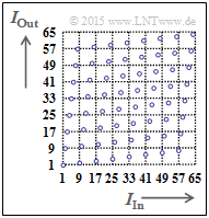
For the following description of the interleavers we use the assignment $I_{\rm In} → I_{\rm Out}$. These labels stand for the indices of output and input sequence, respectively. The interleaver variable is named $I_{\rm max}$ .
There are several, fundamentally different interleaver concepts:
⇒ In a »block interleaver« one fills a matrix with $N_{\rm C}$ columns and $N_{\rm R}$ rows column-by-column and reads the matrix row-by-row. Thus an information block with $I_{\rm max} = N_{\rm C} \cdot N_{\rm R}$ bit is deterministically scrambled.
The right graph illustrates the principle for $I_{\rm max} = 64$ ⇒ $1 ≤ I_{\rm In} \le 64$ and $1 ≤ I_{\rm Out} \le 64$. The order of the output bits is then:
- $$1, 9, 17, 25, 33, 41, 49, 57, 2, 10, 18, \ \text{...}\hspace{0.05cm} , 48, 56, 64.$$
More information on block interleaving is available in the "Exercise 4.8Z".
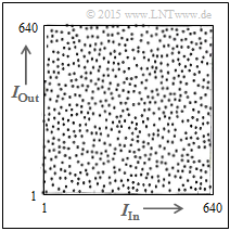
⇒ Turbo codes often use the »$S$–random interleaver«. This pseudo random algorithm with the parameter "$S$" guarantees
- that two indices less than $S$ apart at the input
- occur at least at the distance $S + 1$ at the output.
The left graph shows the $S$–random characteristic $I_{\rm Out}(I_{\rm In})$ for $I_{\rm max} = 640$.
- This algorithm is also deterministic, and one can undo the scrambling in the decoder ⇒ "De–interleaving".
- The distribution still seems "more random" than with block interleaving.
Bit-wise iterative decoding of a turbo code
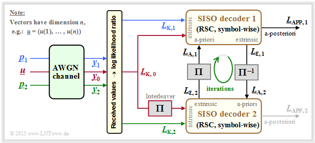
The decoding of a turbo code is basically done as described in section "Bit-wise Soft–in Soft–out Decoding". From the following graphic, however, you can also see some special features that apply only to the turbo decoder.
Assumed is a rate $1/3$ turbo code according to the description in the "first section of this page". Also, the color scheme for the information sequence $\underline{u}$ and the two parity sequences $\underline{p}_1$ and $\underline{p}_2$ are adapted from the earlier graphics. Further, it should be noted:
- The received vectors $\underline{y}_0,\hspace{0.15cm} \underline{y}_1,\hspace{0.15cm} \underline{y}_2$ are real-valued and provide the respective soft information with respect to the information sequence $\underline{u}$ and the sequences $\underline{p}_1$ $($parity for encoder 1$)$ and $\underline{p}_2$ $($parity for encoder 2$)$.
- The decoder 1 receives the required intrinsic information in the form of the $L$ values $L_{\rm K,\hspace{0.03cm} 0}$ $($out $\underline{y}_0)$ and $L_{\rm K,\hspace{0.03cm}1}$ $($out $\underline{y}_1)$ over each bit of the sequences $\underline{u}$ and $\underline{p}_1$.
- In the second decoder, the scrambling of the information sequence $\underline{u}$ must be taken into account. Thus, the $L$ values to be processed are $\pi(L_{\rm K, \hspace{0.03cm}0})$ and $L_{\rm K, \hspace{0.03cm}2}$.
- In the general $\text{SISO decoder}$ the information exchange between the two component decoders was controlled with $\underline{L}_{\rm A, \hspace{0.03cm}2} = \underline{L}_{\rm E, \hspace{0.03cm}1}$ and $\underline{L}_{\rm A, \hspace{0.03cm}1} = \underline{L}_{\rm E, \hspace{0.03cm}2}$.
- Written out at the bit level, these equations are denoted by $(1 ≤ i ≤ n)$:
- \[L_{\rm A, \hspace{0.03cm}2}(i) = L_{\rm E, \hspace{0.03cm}1}(i) \hspace{0.5cm}{\rm resp.}\hspace{0.5cm} L_{\rm A, \hspace{0.03cm}1}(i) = L_{\rm E, \hspace{0.03cm}2}(i) \hspace{0.03cm}.\]
- In the case of the turbo decoder, the interleaver must also be taken into account in this information exchange. Then for $i = 1, \ \text{...}\hspace{0.05cm} , \ n$:
- \[L_{\rm A, \hspace{0.03cm}2}\left ({\rm \pi}(i) \right ) = L_{\rm E, \hspace{0.03cm}1}(i) \hspace{0.5cm}{\rm bzw.}\hspace{0.5cm} L_{\rm A, \hspace{0.03cm}1}(i) = L_{\rm E, \hspace{0.03cm}2}\left ({\rm \pi}(i) \right ) \hspace{0.05cm}.\]
- The a-posteriori $L$ value is $($arbitrarily$)$ given by decoder 1 in the above model. This can be justified by the fact that one iteration stands for a twofold information exchange.
Performance of the turbo codes
We consider, as in the last sections, the rate $1/3$ turbo code
- with equal filter functions $G_1(D) = G_2(D) = (1 + D^2)/(1 + D + D^2)$ ⇒ memory $m = 2$,
- with the interleaver size $K$; first apply $K = 10000,$ and
- a sufficient large number of iterations $(I = 20)$, almost equivalent in result to "$I → ∞$".
The two RSC component codes are each terminated on $K$ bits. Therefore we group
- the information sequence $\underline{u}$ into blocks of $K$ information bits each, and
- the encoded sequence $\underline{x}$ to blocks with each $N = 3 \cdot K$ encoded bits.
All results apply to the $\text{AWGN channel}$. Data are taken from the lecture notes [Liv15][1].
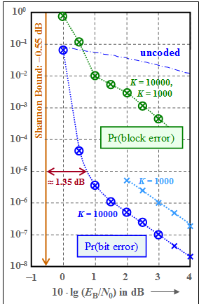
The graph shows as a green curve the »block error probability« ⇒ ${\rm Pr(block\:error)}$ in double logarithmic representation depending on the AWGN characteristic $10 \cdot {\rm lg} \, (E_{\rm B}/N_0)$. It can be seen:
- The points marked with crosses resulted from the weight functions of the turbo code using the $\text{Union Bound}$. The simulation results – in the graph marked by circles – are almost congruent with the analytically calculated values.
- The "Union Bound" is only an upper bound based on maximum likelihood decoding $\rm (ML)$. The iterative decoder is suboptimal (i.e., worse than "maximum likelihood"). These two effects seem to almost cancel each other out.
- At $10 \cdot {\rm lg} \, (E_{\rm B}/N_0) = 1 \ \rm dB$ there is a kink in the (green) curve, corresponding to the slope change of ${\rm Pr(bit\:error)}$ ⇒ blue curve.
The blue crosses $($"calculation"$)$ and the blue circles $($"simulation"$)$ denote the »bit error probability« for the interleaver size $K = 10000$. The (dash-dotted) curve for uncoded transmission is drawn as a comparison curve.
⇒ To these blue curves is to be noted:
- For small abscissa values, the curve slope in the selected plot is nearly linear and sufficiently steep. For example, for ${\rm Pr(bit\, error)} = 10^{-5}$ one needs at least $10 \cdot {\rm lg} \, (E_{\rm B}/N_0) \approx \, 0.8 \ \rm dB$.
- Compared to the $\text{Shannon bound}$, which results for code rate $R = 1/3$ to $10 \cdot {\rm lg} \, (E_{\rm B}/N_0) \approx \, –0.55 \ \rm dB$, our standard turbo code $($with memory $m = 2)$ is only about $1.35 \ \rm dB$ away.
- From $10 \cdot {\rm lg} \, (E_{\rm B}/N_0) \approx 0.5 \ \rm dB$ the curve runs flatter. From $\approx 1.5 \ \rm dB$ the curve is again (nearly) linear with lower slope. For ${\rm Pr(bit\:error)} = 10^{-7}$ one needs about $10 \cdot {\rm lg} \, (E_{\rm B}/N_0) = 3 \ \rm dB$.
⇒ We now try to explain the flatter drop in bit error probability with larger $E_{\rm B}/N_0$. This is called an »$\text{error floor}$«:
- The reason for this asymptotically worse behavior with better channel $($in the example: from $10 \cdot {\rm lg} \, E_{\rm B}/N_0 \ge 2 \ \rm dB)$ is the period $P$ of the encoder impulse response $\underline{g}$, as demonstrated in the section $\rm Interleaving$, and explained in the "Exercise 4.10" with examples.
- For $m = 2$, the period is $P = 2^m -1 = 3$. Thus, for $\underline{u} = (1, 1, 1) ⇒ w_{\rm H}(\underline{u}) = 3$ the parity sequence is bounded: $\underline{p} = (1, 0, 1)$ ⇒ $w_{\rm H}(\underline{p}) = 2$ despite unbounded impulse response $\underline{g}$.
- The sequence $\underline{u} = (0, \ \text{...}\hspace{0.05cm} , \ 0, \ 1, \ 0, \ 0, \ 1, \ 0, \ \text{...}\hspace{0.05cm})$ ⇒ $U(D) = D^x \cdot (1 + D^P)$ also leads to a small Hamming weight $w_{\rm H}(\underline{p})$ at the output, which complicates the iterative decoding process.
- Some workaround is provided by the interleaver, which ensures that both sequences $\underline{p}_1$ and $\underline{p}_2$ are not simultaneously loaded by very small Hamming weights $w_{\rm H}(\underline{p}_1)$ and $w_{\rm H}(\underline{p}_2)$.
- From the graph you can also see that the bit error probability is inversely proportional to the interleaver size $K$. That means: With large $K$ the despreading of unfavorable input sequences works better.
- However, the approximation $K \cdot {\rm Pr(bit\:error) = const.}$ is valid only for larger $E_{\rm B}/N_0$ values ⇒ small bit error probabilities. The described effect also occurs for smaller $E_{\rm B}/N_0$ values, but then the effects on the bit error probability are smaller.
- The flatter shape of the block error probability $($green curve$)$ holds largely independent of the interleaver size $K$, i.e., for $K = 1000$ as well as for $K = 10000$. In the range $10 \cdot {\rm lg} \, E_{\rm B}/N_0 > 2 \ \rm dB$ namely single errors dominate, so that here the approximation ${\rm Pr(block\: error)} \approx {\rm Pr(bit\:error)} \cdot K$ is valid.
$\text{Conclusions:}$ The exemplary shown bit error probability and block error probability curves also apply qualitatively for $m > 2$, e.g. for the UMTS and LTE turbo codes $($each with $m = 3)$, which is analyzed in "Exercise 4.10". However, some quantitative differences emerge:
- The curve is steeper for small $E_{\rm B}/N_0$ and the distance from the Shannon bound is slightly less than in the example shown here for $m = 2$.
- Also for larger $m$ there is an "error floor". However, the kink in the displayed curves then occurs later, i.e. at smaller error probabilities.
Serial concatenated turbo codes – SCCC
The turbo codes considered so far are sometimes referred to as "parallel concatenated convolutional codes" $\rm (PCCC)$.
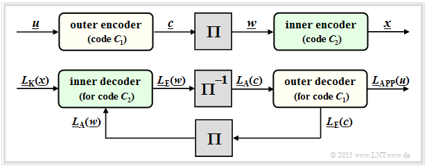
Some years after Berrou's invention, "serial concatenated convolutional codes" $\rm (SCCC)$ were also proposed by other authors according to the following diagram.
- The information sequence $\underline{u}$ is located at the outer convolutional encoder $\mathcal{C}_1$. Let its output sequence be $\underline{c}$.
- After the interleaver $(\Pi)$ follows the inner convolutional encoder $\mathcal{C}_2$. The encoded sequence is called $\underline{x}$ .
- The resulting code rate is $R = R_1 \cdot R_2$. For rate $1/2$ component codes: $R = 1/4$.
The bottom diagram shows the SCCC decoder and illustrates the processing of $L$–values and the exchange of extrinsic information between the two component decoders:
- The inner decoder $($code $\mathcal{C}_2)$ receives the intrinsic information $\underline{L}_{\rm K}(\underline{x})$ from the channel and a-priori information $\underline{L}_{\rm A}(\underline{w})$ with $\underline{w} = \pi(\underline{c})$ from the outer decoder $($after interleaving$)$ and delivers the extrinsic information $\underline{L}_{\rm E}(\underline{w})$ to the outer decoder.
- The outer decoder $(\mathcal{C}_1)$ processes the a-priori information $\underline{L}_{\rm A}(\underline{c})$, i.e. the extrinsic information $\underline{L}_{\rm E}(\underline{w})$ after de–interleaving. It provides the extrinsic information $\underline{L}_{\rm E}(\underline{c})$.
- After a sufficient number of iterations, the desired decoding result is obtained in the form of the a-posteriori $L$–values $\underline{L}_{\rm APP}(\underline{u})$ of the information sequence $\underline{u}$.
$\text{Conclusions:}$ Important for serial concatenated convolutional codes $\rm (SCCC)$ is that the inner code $\mathcal{C}_2$ is recursive $($i.e. a RSC code$)$. The outer code $\mathcal{C}_1$ may also be non-recursive.
Regarding the performance of such codes, it should be noted:
- An SCCC is often better than a PCCC ⇒ lower error floor for large $E_{\rm B}/N_0$. The statement is already true for SCCC component codes with memory $m = 2$ $($only four trellis states$)$, while for PCCC the memory $m = 3$ and $m = 4$ $($eight and sixteen trellis states, respectively$)$ should be.
- In the lower range $($small $E_{\rm B}/N_0)$ on the other hand, the best serial concatenated convolutional code is several tenths of a decibel worse than the comparable turbo code according to Berrou $\rm (PCCC)$. The distance from the Shannon bound is correspondingly larger.
Some application areas for turbo codes
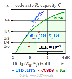
Turbo codes are used in almost all newer communication systems. The graph shows their performance with the AWGN channel compared to $\text{Shannon's channel capacity}$ $($blue curve$)$.
The green highlighted area "BPSK" indicates the Shannon bound for digital systems with binary input, with which according to the $\text{channel coding theorem}$ an error-free transmission is just possible.
It should be noted that the bit error rate $\rm BER= 10^{-5}$ is the basis here for the channel codes of standardized systems which are drawn in, while the information-theoretical capacity curves $($Shannon, BPSK$)$ apply to the error probability $0$.
- The blue rectangles mark the turbo codes for UMTS. These are rate $1/3$ codes with memory $m = 3$. The performance depends strongly on the interleaver size. With $K = 6144$ this code is only about $1 \rm dB$ to the right of the Shannon bound. LTE uses the same turbo codes. Minor differences occur due to the different interleaver.
- The red crosses mark the turbo codes according to $\rm CCSDS$ $($"Consultative Committee for Space Data Systems"$)$, developed for use in space missions. This class assumes the fixed interleaver size $K = 6920$ and provides codes of rate $1/6$, $1/4$, $1/3$ and $1/2$. The lowest code rates allow operation at $10 \cdot {\rm lg} \, (E_{\rm B}/N_0) \approx 0 \ \rm dB$.
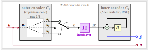
- The green circle represents a very simple "Repeat Accumulate" $\rm (RA)$ code, a serial concatenated turbo code. The following is an outline of its structure: The outer decoder uses a $\text{repetition code}$, in the drawn example with rate $R = 1/3$. The interleaver is followed by an RSC code with $G(D) = 1/(1 + D)$ ⇒ memory $m = 1$. When executed systematically, the total code rate is $R = 1/4$ $($three parity bits are added to each bit of information$)$.
- From the graph on the top right, one can see that this simple RA code is surprisingly good.
- With the interleaver size $K = 300000$ the distance from the Shannon bound is only about $1.5 \ \rm dB$ $($green dot$)$.
- Similar repeat accumulate codes are provided for the "DVB Return Channel Terrestrial" $\rm (RCS)$ standard and for the WiMax standard $\rm (IEEE 802.16)$.
Exercises for the chapter
Exercise 4.08: Repetition to the Convolutional Codes
Exercise 4.08Z: Basics about Interleaving
Exercise 4.09: Recursive Systematic Convolutional Codes
Exercise 4.10: Turbo Enccoder for UMTS and LTE
References
- ↑ Liva, G.: Channels Codes for Iterative Decoding. Lecture notes, Department of Communications Engineering, TU Munich and DLR Oberpfaffenhofen, 2015.


