Difference between revisions of "Mobile Communications/General Description of Time Variant Systems"
| (64 intermediate revisions by 5 users not shown) | |||
| Line 1: | Line 1: | ||
{{Header | {{Header | ||
| − | |Untermenü= | + | |Untermenü=Frequency-Selective Transmission Channels |Vorherige Seite=Non-Frequency Selective Fading With Direct Component |
| − | |Vorherige Seite= | + | |Nächste Seite=Multipath Reception in Mobile Communications}} |
| − | |Nächste Seite= | ||
| − | }} | ||
| − | == | + | == # OVERVIEW OF THE SECOND MAIN CHAPTER # == |
<br> | <br> | ||
| − | + | After the time variance, the term »'''frequency selectivity'''« is now introduced and illustrated with examples, a channel property which is also of great importance for mobile communications. As in the entire book, the description is given in the equivalent low-pass range. | |
| − | + | It is covered in detail: | |
| − | |||
| − | |||
| − | + | #The »difference between time-invariant and time-variant systems«, | |
| + | #the »time-variant impulse response« as an important descriptive function of time-variant systems, | ||
| + | #»multi-way reception« as the cause of frequency-selective behaviour, | ||
| + | #a detailed derivation and interpretation of the »GWSSUS channel model«, | ||
| + | #the characteristics of the GWSSUS model: »coherence bandwidth, correlation duration«, etc. | ||
| − | ::<math>r(t) = s(t) \star h(t) \hspace{0.4cm} {\rm | + | |
| + | |||
| + | == Transfer function and impulse response == | ||
| + | <br> | ||
| + | The description parameters of a communication system have already been described in two chapters of the book "Linear Time Variant Systems": | ||
| + | * [[Linear_and_Time_Invariant_Systems/System_Description_in_Frequency_Domain|"System Description in Frequency Domain"]], | ||
| + | * [[Linear_and_Time_Invariant_Systems/System_Description_in_Time_Domain|"System Description in Time Domain"]]. | ||
| + | |||
| + | [[File:EN_Mob_T_2_1_S1_neu.png|right|frame|Considered LTI system|class=fit]] | ||
| + | |||
| + | |||
| + | The most important results are briefly explained again here. We assume a linear and time-invariant system ⇒ $\text{LTI system}$ with the signal $s(t)$ at the input and the output signal $r(t)$. For the sake of simplicity, let $s(t)$ and $r(t)$ be real. Then the following applies: | ||
| + | *The system can be completely characterized by the [[Linear_and_Time_Invariant_Systems/System_Description_in_Frequency_Domain#Frequency_response_.E2.80.93_Transfer_function|$\text{transfer function}$]] $H(f)$ which is also referred to as the "frequency response". By definition :$$H(f) = R(f)/S(f).$$ | ||
| + | |||
| + | *Similarly, the system is defined by the [[Linear_and_Time_Invariant_Systems/System_Description_in_Time_Domain#Impulse_response|$\text{impulse response}$]] $h(t)$ , which is the [[Signal_Representation/Fourier_Transform_and_its_Inverse#The_second_Fourier_integral|$\text{inverse Fourier transform}$]] of $H(f)$. The output signal results from the convolution: | ||
| + | |||
| + | ::<math>r(t) = s(t) \star h(t) \hspace{0.4cm} {\rm with} \hspace{0.4cm} h(t) | ||
\hspace{0.2cm} \circ\!\!-\!\!\!-\!\!\!-\!\!\bullet \hspace{0.2cm} H(f) | \hspace{0.2cm} \circ\!\!-\!\!\!-\!\!\!-\!\!\bullet \hspace{0.2cm} H(f) | ||
\hspace{0.05cm}.</math> | \hspace{0.05cm}.</math> | ||
| − | + | {{BlaueBox|TEXT= | |
| − | * | + | $\text{Definitions:}$ The following input signals are suitable for detecting the linear distortions caused by $H(f)$ or $h(t)$: |
| − | + | *a [[Signal_Representation/Special_Cases_of_Pulses#Dirac_delta_or_impulse|$\text{Dirac delta}$]] or "impulse": | |
| − | + | :$$s(t) = \delta(t) \hspace{0.3cm}\Rightarrow \hspace{0.3cm} r(t) = \delta(t) \star h(t)= h(t)\hspace{0.3cm}\Rightarrow \hspace{0.3cm} \text{impulse response,}$$ | |
| + | *a [[Linear_and_Time_Invariant_Systems/System_Description_in_Time_Domain#Step_response|$\text{step function}$]] or "Heaviside step function": | ||
| + | :$$s(t) = \gamma(t) \hspace{0.3cm}\Rightarrow \hspace{0.35cm} r(t) = \gamma(t) \star h(t)\hspace{1.5cm}\Rightarrow \hspace{0.3cm} \text{step response,}$$ | ||
| + | *a [[Signal_Representation/Discrete-Time_Signal_Representation#Dirac_comb_in_time_and_frequency_domain|$\text{Dirac comb}$]] or "Dirac delta train": | ||
| + | :$$s(t) = p_\delta(t) \hspace{0.25cm}\Rightarrow \hspace{0.3cm} r(t) = p_\delta(t) \star h(t)\hspace{1.3cm}\Rightarrow \hspace{0.3cm} \text{impulse response train.}$$}} | ||
| + | |||
| + | |||
| + | On the other hand, a DC signal $s(t) = A$ is not suitable to make the frequency dependence of the LTI system visible: <br> ⇒ With a low-pass system the output signal would then be always constant, independent of $H(f)$: $r(t) = A \cdot H(f= 0)$.<br> | ||
| − | + | In the next section we consider a Dirac delta train $p_\delta(t)$ as an input signal $s(t)$: <br> ⇒ Hereby the similarities and differences between time-invariant and time-variant systems can be shown clearly.<br> | |
| − | + | <i>Note:</i> The properties of $H(f)$ and $h(t)$ are covered in detail in the $\text{LNTwww learning video}$ (in German language):<br> | |
| + | [https://www.lntwww.de/Eigenschaften_des_%C3%9Cbertragungskanals_(Lernvideo) "Eigenschaften des Übertragungskanals"] ⇒ "Some remarks on the transfer function".<br> | ||
| − | |||
| − | == | + | == Time–invariant vs. time–variant channels == |
<br> | <br> | ||
| − | + | The graphic is intended to illustrate the difference between a linear time–invariant channel $\rm (LTI)$ and a linear time–variant channel $\rm (LTV)$ .<br> | |
| − | [[File: | + | [[File:EN_Mob_T_2_1_S2.png|right|frame|Time–invariant and time–variant channel|class=fit]] |
| − | + | One can see from this illustration: | |
| − | * | + | *The transmitted signal $s(t)$ is a Dirac delta train $p_\delta(t)$, i.e. an infinite sequence of Dirac deltas in equidistant intervals $T$, all with the weight $1$ (see upper graph): |
::<math>s(t) = p_{\rm \delta} (t) = \sum_{n = -\infty}^{+\infty} {\rm \delta} (t - n \cdot T) | ::<math>s(t) = p_{\rm \delta} (t) = \sum_{n = -\infty}^{+\infty} {\rm \delta} (t - n \cdot T) | ||
\hspace{0.05cm}.</math> | \hspace{0.05cm}.</math> | ||
| − | * | + | *The Dirac delta at $t = 0$ is marked in green. The signal at the channel output is equal to $r(t) = h(t)$ , with $s(t) = {\rm \delta}(t)$ , also indicated in green. As a condition, it is assumed that the extension of the impulse response $h(t)$ is smaller than $T$.<br>. |
| − | * | + | *The entire received signal after the LTI channel, according to the middle graph, can then be written as: |
::<math>r(t) = p_{\rm \delta} (t) \star h(t) = \sum_{n = -\infty}^{+\infty} h (t - n \cdot T) | ::<math>r(t) = p_{\rm \delta} (t) \star h(t) = \sum_{n = -\infty}^{+\infty} h (t - n \cdot T) | ||
\hspace{0.05cm}.</math> | \hspace{0.05cm}.</math> | ||
| − | * | + | *For a time-variant channel (lower graph) this equation is not applicable. In each time interval, a (slightly) different signal shape is obtained. |
| + | |||
| + | |||
| + | {{BlaueBox|TEXT= | ||
| + | $\text{Conclusion:}$ With a »'''time-variant channel'''« you cannot specify neither a one-parameter impulse response $h(t)$ nor a transfer function $H(f)$ .}}<br> | ||
| + | |||
| + | <i>Note:</i> The differences between LTI and LTV systems are clarified with the $\text{LNTwww learning video}$ (in German language):<br> | ||
| + | [https://www.lntwww.de/Eigenschaften_des_%C3%9Cbertragungskanals_(Lernvideo) "Eigenschaften des Übertragungskanals"] ⇒ "Some remarks on the transfer function".<br> | ||
| − | |||
| − | == | + | == Two-dimensional impulse response== |
<br> | <br> | ||
| − | + | [[File:EN_Mob_T_2_1_S3.png|right|frame|Two-dimensional impulse response|class=fit]] | |
| + | |||
| + | To identify a time-variant impulse response, a second parameter is used and the impulse response is preferably mapped in a three-dimensional coordinate system.<br> | ||
| + | |||
| + | The condition for this is that the channel is still linear. One speaks then of a $\text{LTV system}$ ("linear time-variant"). | ||
| − | + | The following relations apply: | |
| − | |||
| − | ::<math>\text{ | + | ::<math>\text{LTI:}\hspace{0.5cm} r(t) = \int_{-\infty}^{+\infty} h(\tau) \cdot s(t-\tau) \hspace{0.15cm}{\rm d}\tau \hspace{0.05cm},</math> |
| − | ::<math>\text{ | + | ::<math>\text{LTV:}\hspace{0.5cm} r(t) \hspace{-0.1cm} = \hspace{-0.1cm} \int_{-\infty}^{+\infty} h(\tau, \hspace{0.1cm}t) \cdot s(t-\tau) \hspace{0.15cm}{\rm d}\tau \hspace{0.05cm}.</math> |
<br clear=all> | <br clear=all> | ||
| − | + | Regarding the last equation and the above graph, it should be noted | |
| − | * | + | *The parameter $\tau$ specifies the »'''delay time'''« to denote the time dispersion. By writing out the convolution operation, it was possible to make $\tau$ also the parameter of the LTI impulse response. In the last sections we spoke about $h(t)$ .<br> |
| − | * | + | *The second parameter of the impulse response or the second axis marks the »'''absolute time'''« $t$, which is used, among other things, to describe the time variance. At different times $t$ the impulse response $h(\tau, \hspace{0.05cm}t)$ has a different form.<br> |
| − | * | + | *A peculiarity of the 2D representation is that the $t$–axis is always plotted discrete-timely $($at multiples of $T)$ while the $\tau$–axis can be continuous in time as in the example shown. However, in mobile communications, a discrete-time $h(\tau, \hspace{0.05cm}t_0)$ with respect to $\tau$ is assumed $($"echoes"$)$. |
| − | * | + | *The LTV equation is only applicable if the change of the channel $($marked in the figure by the parameter $T)$ proceeds slowly in comparison to the maximum delay $\tau_{\rm max}$. In mobile communications this condition ⇒ $\tau_{\rm max} < T$ is almost always fulfilled. |
| − | * | + | *Selecting whether to apply the first Fourier integral to the parameter $\tau$ or $t$ leads to different spectral functions. In the [[Aufgaben:Exercise 2.1Z: 2D-Frequency and 2D-Time Representations|"Exercise 2.1Z"]] for example, the time-variant »'''two-dimensional transfer function'''« is considered: |
::<math>H(f,\hspace{0.05cm} t) | ::<math>H(f,\hspace{0.05cm} t) | ||
| Line 82: | Line 114: | ||
| − | == | + | ==Exercises for the chapter== |
| − | [[Aufgaben:2.1 | + | [[Aufgaben:Exercise 2.1: Two-Dimensional Impulse Response]] |
| + | |||
| + | [[Aufgaben:Exercise 2.1Z: 2D-Frequency and 2D-Time Representations]] | ||
| + | |||
| − | |||
{{Display}} | {{Display}} | ||
Latest revision as of 15:41, 29 January 2023
Contents
# OVERVIEW OF THE SECOND MAIN CHAPTER #
After the time variance, the term »frequency selectivity« is now introduced and illustrated with examples, a channel property which is also of great importance for mobile communications. As in the entire book, the description is given in the equivalent low-pass range.
It is covered in detail:
- The »difference between time-invariant and time-variant systems«,
- the »time-variant impulse response« as an important descriptive function of time-variant systems,
- »multi-way reception« as the cause of frequency-selective behaviour,
- a detailed derivation and interpretation of the »GWSSUS channel model«,
- the characteristics of the GWSSUS model: »coherence bandwidth, correlation duration«, etc.
Transfer function and impulse response
The description parameters of a communication system have already been described in two chapters of the book "Linear Time Variant Systems":
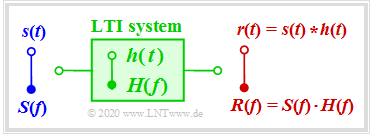
The most important results are briefly explained again here. We assume a linear and time-invariant system ⇒ $\text{LTI system}$ with the signal $s(t)$ at the input and the output signal $r(t)$. For the sake of simplicity, let $s(t)$ and $r(t)$ be real. Then the following applies:
- The system can be completely characterized by the $\text{transfer function}$ $H(f)$ which is also referred to as the "frequency response". By definition :$$H(f) = R(f)/S(f).$$
- Similarly, the system is defined by the $\text{impulse response}$ $h(t)$ , which is the $\text{inverse Fourier transform}$ of $H(f)$. The output signal results from the convolution:
- \[r(t) = s(t) \star h(t) \hspace{0.4cm} {\rm with} \hspace{0.4cm} h(t) \hspace{0.2cm} \circ\!\!-\!\!\!-\!\!\!-\!\!\bullet \hspace{0.2cm} H(f) \hspace{0.05cm}.\]
$\text{Definitions:}$ The following input signals are suitable for detecting the linear distortions caused by $H(f)$ or $h(t)$:
- a $\text{Dirac delta}$ or "impulse":
- $$s(t) = \delta(t) \hspace{0.3cm}\Rightarrow \hspace{0.3cm} r(t) = \delta(t) \star h(t)= h(t)\hspace{0.3cm}\Rightarrow \hspace{0.3cm} \text{impulse response,}$$
- a $\text{step function}$ or "Heaviside step function":
- $$s(t) = \gamma(t) \hspace{0.3cm}\Rightarrow \hspace{0.35cm} r(t) = \gamma(t) \star h(t)\hspace{1.5cm}\Rightarrow \hspace{0.3cm} \text{step response,}$$
- a $\text{Dirac comb}$ or "Dirac delta train":
- $$s(t) = p_\delta(t) \hspace{0.25cm}\Rightarrow \hspace{0.3cm} r(t) = p_\delta(t) \star h(t)\hspace{1.3cm}\Rightarrow \hspace{0.3cm} \text{impulse response train.}$$
On the other hand, a DC signal $s(t) = A$ is not suitable to make the frequency dependence of the LTI system visible:
⇒ With a low-pass system the output signal would then be always constant, independent of $H(f)$: $r(t) = A \cdot H(f= 0)$.
In the next section we consider a Dirac delta train $p_\delta(t)$ as an input signal $s(t)$:
⇒ Hereby the similarities and differences between time-invariant and time-variant systems can be shown clearly.
Note: The properties of $H(f)$ and $h(t)$ are covered in detail in the $\text{LNTwww learning video}$ (in German language):
"Eigenschaften des Übertragungskanals" ⇒ "Some remarks on the transfer function".
Time–invariant vs. time–variant channels
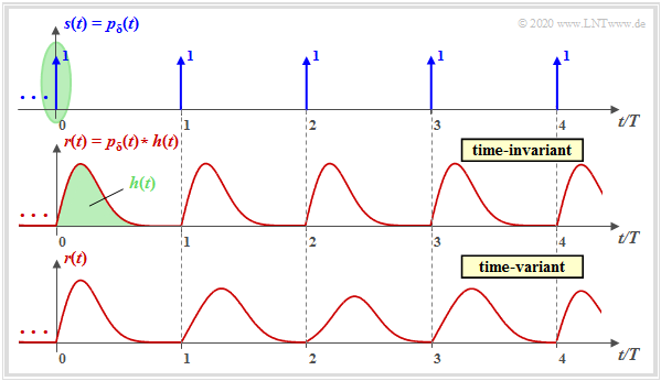
The graphic is intended to illustrate the difference between a linear time–invariant channel $\rm (LTI)$ and a linear time–variant channel $\rm (LTV)$ .
One can see from this illustration:
- The transmitted signal $s(t)$ is a Dirac delta train $p_\delta(t)$, i.e. an infinite sequence of Dirac deltas in equidistant intervals $T$, all with the weight $1$ (see upper graph):
- \[s(t) = p_{\rm \delta} (t) = \sum_{n = -\infty}^{+\infty} {\rm \delta} (t - n \cdot T) \hspace{0.05cm}.\]
- The Dirac delta at $t = 0$ is marked in green. The signal at the channel output is equal to $r(t) = h(t)$ , with $s(t) = {\rm \delta}(t)$ , also indicated in green. As a condition, it is assumed that the extension of the impulse response $h(t)$ is smaller than $T$.
.
- The entire received signal after the LTI channel, according to the middle graph, can then be written as:
- \[r(t) = p_{\rm \delta} (t) \star h(t) = \sum_{n = -\infty}^{+\infty} h (t - n \cdot T) \hspace{0.05cm}.\]
- For a time-variant channel (lower graph) this equation is not applicable. In each time interval, a (slightly) different signal shape is obtained.
$\text{Conclusion:}$ With a »time-variant channel« you cannot specify neither a one-parameter impulse response $h(t)$ nor a transfer function $H(f)$ .
Note: The differences between LTI and LTV systems are clarified with the $\text{LNTwww learning video}$ (in German language):
"Eigenschaften des Übertragungskanals" ⇒ "Some remarks on the transfer function".
Two-dimensional impulse response
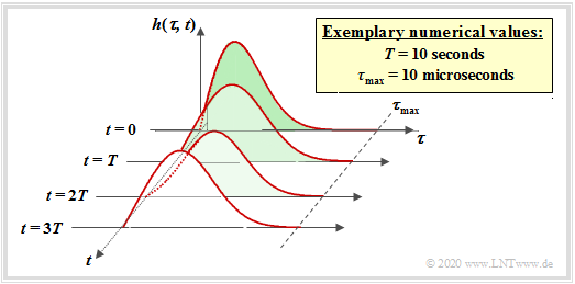
To identify a time-variant impulse response, a second parameter is used and the impulse response is preferably mapped in a three-dimensional coordinate system.
The condition for this is that the channel is still linear. One speaks then of a $\text{LTV system}$ ("linear time-variant").
The following relations apply:
- \[\text{LTI:}\hspace{0.5cm} r(t) = \int_{-\infty}^{+\infty} h(\tau) \cdot s(t-\tau) \hspace{0.15cm}{\rm d}\tau \hspace{0.05cm},\]
- \[\text{LTV:}\hspace{0.5cm} r(t) \hspace{-0.1cm} = \hspace{-0.1cm} \int_{-\infty}^{+\infty} h(\tau, \hspace{0.1cm}t) \cdot s(t-\tau) \hspace{0.15cm}{\rm d}\tau \hspace{0.05cm}.\]
Regarding the last equation and the above graph, it should be noted
- The parameter $\tau$ specifies the »delay time« to denote the time dispersion. By writing out the convolution operation, it was possible to make $\tau$ also the parameter of the LTI impulse response. In the last sections we spoke about $h(t)$ .
- The second parameter of the impulse response or the second axis marks the »absolute time« $t$, which is used, among other things, to describe the time variance. At different times $t$ the impulse response $h(\tau, \hspace{0.05cm}t)$ has a different form.
- A peculiarity of the 2D representation is that the $t$–axis is always plotted discrete-timely $($at multiples of $T)$ while the $\tau$–axis can be continuous in time as in the example shown. However, in mobile communications, a discrete-time $h(\tau, \hspace{0.05cm}t_0)$ with respect to $\tau$ is assumed $($"echoes"$)$.
- The LTV equation is only applicable if the change of the channel $($marked in the figure by the parameter $T)$ proceeds slowly in comparison to the maximum delay $\tau_{\rm max}$. In mobile communications this condition ⇒ $\tau_{\rm max} < T$ is almost always fulfilled.
- Selecting whether to apply the first Fourier integral to the parameter $\tau$ or $t$ leads to different spectral functions. In the "Exercise 2.1Z" for example, the time-variant »two-dimensional transfer function« is considered:
- \[H(f,\hspace{0.05cm} t) \hspace{0.2cm} \bullet\!\!-\!\!\!-\!\!\!-\!\!\circ \hspace{0.2cm} h(\tau,\hspace{0.05cm}t) \hspace{0.05cm}.\]
Exercises for the chapter
Exercise 2.1: Two-Dimensional Impulse Response
Exercise 2.1Z: 2D-Frequency and 2D-Time Representations


