Difference between revisions of "Applets:PDF, CDF and Moments of Special Distributions"
m (Text replacement - "Biographies_and_Bibliographies/LNTwww_members_from_LNT#Prof._Dr.-Ing._habil._G.C3.BCnter_S.C3.B6der_.28at_LNT_since_1974.29" to "Biographies_and_Bibliographies/LNTwww_members_from_LNT#Prof._Dr.-Ing._habil._G.C3.BCnter_S.C3.B6der_.28at_LNT_from_1974-2024.29") |
|||
| (10 intermediate revisions by 3 users not shown) | |||
| Line 15: | Line 15: | ||
In addition, some integral parameters are output, namely | In addition, some integral parameters are output, namely | ||
*the linear mean value $m_X = {\rm E}\big[X \big]$, | *the linear mean value $m_X = {\rm E}\big[X \big]$, | ||
| − | *the | + | *the second order moment $P_X ={\rm E}\big[X^2 \big] $, |
*the variance $\sigma_X^2 = P_X - m_X^2$, | *the variance $\sigma_X^2 = P_X - m_X^2$, | ||
*the standard deviation $\sigma_X$, | *the standard deviation $\sigma_X$, | ||
| Line 146: | Line 146: | ||
===Gaussian distributed random variables=== | ===Gaussian distributed random variables=== | ||
| − | [[File: | + | [[File:EN_Sto_T_3_5_S2_v2.png |right|frame|Gaussian random variable: PDF and CDF]] |
'''(1)''' »'''Probability density function'''« $($axisymmetric around $m_X)$ | '''(1)''' »'''Probability density function'''« $($axisymmetric around $m_X)$ | ||
:$$f_X(x) = \frac{1}{\sqrt{2\pi}\cdot\sigma_X}\cdot {\rm e}^{-(X-m_X)^2 /(2\sigma_X^2) }.$$ | :$$f_X(x) = \frac{1}{\sqrt{2\pi}\cdot\sigma_X}\cdot {\rm e}^{-(X-m_X)^2 /(2\sigma_X^2) }.$$ | ||
| Line 293: | Line 293: | ||
===Brief description of other distributions=== | ===Brief description of other distributions=== | ||
<br> | <br> | ||
| − | $\text{(A) Rayleigh distribution}$ [[Mobile_Communications/ | + | $\text{(A) Rayleigh distribution}$ [[Mobile_Communications/Probability_Density_of_Rayleigh_Fading|$\text{More detailed description}$]] |
*Probability density function: | *Probability density function: | ||
| Line 305: | Line 305: | ||
| − | $\text{(B) Rice distribution}$ [[Mobile_Communications/ | + | $\text{(B) Rice distribution}$ [[Mobile_Communications/Non-Frequency-Selective_Fading_With_Direct_Component|$\text{More detailed description}$]] |
*Probability density function $(\rm I_0$ denotes the modified zero-order Bessel function$)$: | *Probability density function $(\rm I_0$ denotes the modified zero-order Bessel function$)$: | ||
| Line 315: | Line 315: | ||
| − | $\text{(C) Weibull distribution}$ | + | $\text{(C) Weibull distribution}$ [https://en.wikipedia.org/wiki/Weibull_distribution $\text{More detailed description}$] |
*Probability density function: | *Probability density function: | ||
| Line 325: | Line 325: | ||
| − | $\text{(D) Wigner semicircle distribution}$ | + | $\text{(D) Wigner semicircle distribution}$ [https://en.wikipedia.org/wiki/Wigner_semicircle_distribution $\text{More detailed description}$] |
*Probability density function: | *Probability density function: | ||
| Line 332: | Line 332: | ||
0 \end{array} \right.\hspace{0.15cm} | 0 \end{array} \right.\hspace{0.15cm} | ||
\begin{array}{*{1}c} {\rm for}\hspace{0.1cm} |x- m_X|\hspace{-0.05cm} \le \hspace{-0.05cm}R_X, | \begin{array}{*{1}c} {\rm for}\hspace{0.1cm} |x- m_X|\hspace{-0.05cm} \le \hspace{-0.05cm}R_X, | ||
| − | \\ {\rm | + | \\ {\rm for}\hspace{0.1cm} |x- m_X| \hspace{-0.05cm} > \hspace{-0.05cm} R_X \\ \end{array}.$$ |
*Application: PDF of Chebyshev nodes ⇒ zeros of Chebyshev polynomials from numerics. | *Application: PDF of Chebyshev nodes ⇒ zeros of Chebyshev polynomials from numerics. | ||
| Line 349: | Line 349: | ||
| − | $\text{(F) Cauchy distribution}$ [[Theory_of_Stochastic_Signals/ | + | $\text{(F) Cauchy distribution}$ [[Theory_of_Stochastic_Signals/Further_Distributions#Cauchy_PDF|$\text{More detailed description}$]] |
*Probability density function and distribution function: | *Probability density function and distribution function: | ||
| Line 382: | Line 382: | ||
{{BlueBox|TEXT= | {{BlueBox|TEXT= | ||
| − | '''(3)''' Same settings as before. How must the standard deviation $\sigma_X$ be changed so that with the same mean $m_X$ it holds for the | + | '''(3)''' Same settings as before. How must the standard deviation $\sigma_X$ be changed so that with the same mean $m_X$ it holds for the second order moment: $P_X=2$ ?}} |
* According to Steiner's theorem: $P_X=m_X^2 + \sigma_X^2$ ⇒ $\sigma_X^2 = P_X-m_X^2 = 2 - 1^2 = 1 $ ⇒ $\sigma_X = 1$. | * According to Steiner's theorem: $P_X=m_X^2 + \sigma_X^2$ ⇒ $\sigma_X^2 = P_X-m_X^2 = 2 - 1^2 = 1 $ ⇒ $\sigma_X = 1$. | ||
| Line 470: | Line 470: | ||
<br> | <br> | ||
[[File:Bildschirm_WDF_VTF_neu.png|right|600px|frame|Screenshot of the German version]] | [[File:Bildschirm_WDF_VTF_neu.png|right|600px|frame|Screenshot of the German version]] | ||
| − | '''(A)''' | + | '''(A)''' Selection of the distribution $f_X(x)$ (red curves and output values) |
| − | '''(B)''' | + | '''(B)''' Parameter input for the "red distribution" via slider |
| − | '''(C)''' | + | '''(C)''' Selection of the distribution $f_Y(y)$ (blue curves and output values) |
| − | '''(D)''' | + | '''(D)''' Parameter input for the "red distribution" via slider |
| − | '''(E)''' | + | '''(E)''' Graphic area for the probability density function (PDF) |
| − | '''(F)''' | + | '''(F)''' Graphic area for the distribution function (CDF) |
| − | '''(G)''' | + | '''(G)''' Numerical output for the "red distribution" |
| − | '''(H)''' | + | '''(H)''' Numerical output for the "blue distribution" |
| − | '''( I )''' | + | '''( I )''' Input of $x_*$ and $y_*$ abscissa values for the numerics outputs |
| − | '''(J)''' | + | '''(J)''' Experiment execution area: task selection |
| − | '''(K)''' | + | '''(K)''' Experiment execution area: task description |
| − | '''( L)''' | + | '''( L)''' Experiment execution area: sample solution |
<br> | <br> | ||
| − | ''' | + | '''Selection options for''' for $\rm A$ and $\rm C$: |
| − | + | Gaussian distribution, uniform distribution, triangular distribution, exponential distribution, Laplace distribution, Rayleigh distribution, Rice distribution, Weibull distribution, Wigner semicircle distribution, Wigner parabolic distribution, Cauchy distribution. | |
| − | + | The following »'''integral parameters'''« are output $($with respect to $X)$: | |
| − | + | Linear mean value $m_X = {\rm E}\big[X \big]$, second order moment $P_X ={\rm E}\big[X^2 \big] $, variance $\sigma_X^2 = P_X - m_X^2$, standard deviation $\sigma_X$, Charlier's skewness $S_X$, kurtosis $K_X$. | |
| Line 515: | Line 515: | ||
<br> | <br> | ||
This interactive calculation tool was designed and implemented at the [https://www.ei.tum.de/en/lnt/home/ $\text{Institute for Communications Engineering}$] at the [https://www.tum.de/en $\text{Technical University of Munich}$]. | This interactive calculation tool was designed and implemented at the [https://www.ei.tum.de/en/lnt/home/ $\text{Institute for Communications Engineering}$] at the [https://www.tum.de/en $\text{Technical University of Munich}$]. | ||
| − | *The first version was created in 2005 by [[Biographies_and_Bibliographies/An_LNTwww_beteiligte_Studierende#Bettina_Hirner_.28Diplomarbeit_LB_2005.29| | + | *The first version was created in 2005 by [[Biographies_and_Bibliographies/An_LNTwww_beteiligte_Studierende#Bettina_Hirner_.28Diplomarbeit_LB_2005.29|»Bettina Hirner«]] as part of her diploma thesis with “FlashMX – Actionscript” (Supervisor: [[Biographies_and_Bibliographies/LNTwww_members_from_LNT#Prof._Dr.-Ing._habil._G.C3.BCnter_S.C3.B6der_.28at_LNT_from_1974-2024.29| »Günter Söder« ]] and [[Biographies_and_Bibliographies/LNTwww_members_from_LNT#Dr.-Ing._Klaus_Eichin_.28at_LNT_from_1972-2011.29| »Klaus Eichin« ]]). |
| − | *In 2019 the program was redesigned via HTML5/JavaScript by [[Biographies_and_Bibliographies/ | + | *In 2019 the program was redesigned via HTML5/JavaScript by [[Biographies_and_Bibliographies/Students_involved_in_LNTwww#Matthias_Niller_.28Ingenieurspraxis_Math_2019.29|»Matthias Niller«]] (Ingenieurspraxis Mathematik, Supervisor: [[Biographies_and_Bibliographies/LNTwww_members_from_LÜT#Dr.-Ing._Benedikt_Leible_.28at_L.C3.9CT_since_2017.29| »Benedikt Leible« ]] and [[Biographies_and_Bibliographies/LNTwww_members_from_LÜT#Dr.-Ing._Tasn.C3.A1d_Kernetzky_.28at_L.C3.9CT_from_2014-2022.29| »Tasnád Kernetzky« ]] ). |
| − | *Last revision and English version 2021 by [[ | + | *Last revision and English version 2021 by [[Biographies_and_Bibliographies/Students_involved_in_LNTwww#Carolin_Mirschina_.28Ingenieurspraxis_Math_2019.2C_danach_Werkstudentin.29|»Carolin Mirschina«]] in the context of a working student activity. |
*The conversion of this applet was financially supported by [https://www.ei.tum.de/studium/studienzuschuesse/ $\text{Studienzuschüsse}$] (TUM Department of Electrical and Computer Engineering). We thank. | *The conversion of this applet was financially supported by [https://www.ei.tum.de/studium/studienzuschuesse/ $\text{Studienzuschüsse}$] (TUM Department of Electrical and Computer Engineering). We thank. | ||
Latest revision as of 15:39, 24 February 2025
Open Applet in new Tab Deutsche Version Öffnen
Contents
Applet Description
The applet presents the description forms of two continuous value random variables $X$ and $Y\hspace{-0.1cm}$. For the red random variable $X$ and the blue random variable $Y$, the following basic forms are available for selection:
- Gaussian distribution, uniform distribution, triangular distribution, exponential distribution, Laplace distribution, Rayleigh distribution, Rice distribution, Weibull distribution, Wigner semicircle distribution, Wigner parabolic distribution, Cauchy distribution.
The following data refer to the random variables $X$. Graphically represented are
- the probability density function $f_{X}(x)$ (above) and
- the cumulative distribution function $F_{X}(x)$ (bottom).
In addition, some integral parameters are output, namely
- the linear mean value $m_X = {\rm E}\big[X \big]$,
- the second order moment $P_X ={\rm E}\big[X^2 \big] $,
- the variance $\sigma_X^2 = P_X - m_X^2$,
- the standard deviation $\sigma_X$,
- the Charlier skewness $S_X$,
- the kurtosis $K_X$.
Definition and Properties of the Presented Descriptive Variables
In this applet we consider only (value–)continuous random variables, i.e. those whose possible numerical values are not countable.
- The range of values of these random variables is thus in general that of the real numbers $(-\infty \le X \le +\infty)$.
- However, it is possible that the range of values is limited to an interval: $x_{\rm min} \le X \le +x_{\rm max}$.
Probability density function (PDF)
For a continuous random variable $X$ the probabilities that $X$ takes on quite specific values $x$ are zero: ${\rm Pr}(X= x) \equiv 0$. Therefore, to describe a continuous random variable, we must always refer to the probability density function – in short $\rm PDF$.
$\text{Definition:}$ The value of the »probability density function« $f_{X}(x)$ at location $x$ is equal to the probability that the instantaneous value of the random variable $x$ lies in an (infinitesimally small) interval of width $Δx$ around $x_\mu$, divided by $Δx$:
- $$f_X(x) = \lim_{ {\rm \Delta} x \hspace{0.05cm}\to \hspace{0.05cm} 0} \frac{ {\rm Pr} \big [x - {\rm \Delta} x/2 \le X \le x +{\rm \Delta} x/2 \big ] }{ {\rm \Delta} x}.$$
This extremely important descriptive variable has the following properties:
- For the probability that the random variable $X$ lies in the range between $x_{\rm u}$ and $x_{\rm o} > x_{\rm u}$:
- $${\rm Pr}(x_{\rm u} \le X \le x_{\rm o}) = \int_{x_{\rm u}}^{x_{\rm o}} f_{X}(x) \ {\rm d}x.$$
- As an important normalization property, this yields for the area under the PDF with the boundary transitions $x_{\rm u} → \hspace{0.1cm} – \hspace{0.05cm} ∞$ and $x_{\rm o} → +∞$:
- $$\int_{-\infty}^{+\infty} f_{X}(x) \ {\rm d}x = 1.$$
Cumulative distribution function (CDF)
The cumulative distribution function – in short $\rm CDF$ – provides the same information about the random variable $X$ as the probability density function.
$\text{Definition:}$ The »cumulative distribution function« $F_{X}(x)$ corresponds to the probability that the random variable $X$ is less than or equal to a real number $x$:
- $$F_{X}(x) = {\rm Pr}( X \le x).$$
The CDF has the following characteristics:
- The CDF is computable from the probability density function $f_{X}(x)$ by integration. It holds:
- $$F_{X}(x) = \int_{-\infty}^{x}f_X(\xi)\,{\rm d}\xi.$$
- Since the PDF is never negative, $F_{X}(x)$ increases at least weakly monotonically, and always lies between the following limits:
- $$F_{X}(x → \hspace{0.1cm} – \hspace{0.05cm} ∞) = 0, \hspace{0.5cm}F_{X}(x → +∞) = 1.$$
- Inversely, the probability density function can be determined from the CDF by differentiation:
- $$f_{X}(x)=\frac{{\rm d} F_{X}(\xi)}{{\rm d}\xi}\Bigg |_{\hspace{0.1cm}x=\xi}.$$
- For the probability that the random variable $X$ is in the range between $x_{\rm u}$ and $x_{\rm o} > x_{\rm u}$ holds:
- $${\rm Pr}(x_{\rm u} \le X \le x_{\rm o}) = F_{X}(x_{\rm o}) - F_{X}(x_{\rm u}).$$
Expected values and moments
The probability density function provides very extensive information about the random variable under consideration. Less, but more compact information is provided by the so-called "expected values" and "moments".
$\text{Definition:}$ The »expected value« with respect to any weighting function $g(x)$ can be calculated with the PDF $f_{\rm X}(x)$ in the following way:
- $${\rm E}\big[g (X ) \big] = \int_{-\infty}^{+\infty} g(x)\cdot f_{X}(x) \,{\rm d}x.$$
Substituting into this equation for $g(x) = x^k$ we get the »moment of $k$-th order«:
- $$m_k = {\rm E}\big[X^k \big] = \int_{-\infty}^{+\infty} x^k\cdot f_{X} (x ) \, {\rm d}x.$$
From this equation follows.
- with $k = 1$ for the first order moment or the (linear) mean:
- $$m_1 = {\rm E}\big[X \big] = \int_{-\infty}^{ \rm +\infty} x\cdot f_{X} (x ) \,{\rm d}x,$$
- with $k = 2$ for the second order moment or the second moment:
- $$m_2 = {\rm E}\big[X^{\rm 2} \big] = \int_{-\infty}^{ \rm +\infty} x^{ 2}\cdot f_{ X} (x) \,{\rm d}x.$$
In relation to signals, the following terms are also common:
- $m_1$ indicates the DC component; with respect to the random quantity $X$ in the following we also write $m_X$.
- $m_2$ corresponds to the signal power $P_X$ (referred to the unit resistance $1 \ Ω$ ) .
For example, if $X$ denotes a voltage, then according to these equations $m_X$ has the unit ${\rm V}$ and the power $P_X$ has the unit ${\rm V}^2.$ If the power is to be expressed in "watts" $\rm (W)$, then $P_X$ must be divided by the resistance value $R$.
Central moments
Of particular importance in statistics in general are the so-called central moments from which many characteristics are derived,
$\text{Definition:}$ The »central moments«, in contrast to the conventional moments, are each related to the mean value $m_1$ in each case. For these, the following applies with $k = 1, \ 2,$ ...:
- $$\mu_k = {\rm E}\big[(X-m_{\rm 1})^k\big] = \int_{-\infty}^{+\infty} (x-m_{\rm 1})^k\cdot f_x(x) \,\rm d \it x.$$
- For mean-free random variables, the central moments $\mu_k$ coincide with the noncentral moments $m_k$.
- The first order central moment is by definition equal to $\mu_1 = 0$.
- The noncentral moments $m_k$ and the central moments $\mu_k$ can be converted directly into each other. With $m_0 = 1$ and $\mu_0 = 1$ it is valid:
- $$\mu_k = \sum\limits_{\kappa= 0}^{k} \left( \begin{array}{*{2}{c}} k \\ \kappa \\ \end{array} \right)\cdot m_\kappa \cdot (-m_1)^{k-\kappa},$$
- $$m_k = \sum\limits_{\kappa= 0}^{k} \left( \begin{array}{*{2}{c}} k \\ \kappa \\ \end{array} \right)\cdot \mu_\kappa \cdot {m_1}^{k-\kappa}.$$
Some Frequently Used Central Moments
From the last definition the following additional characteristics can be derived:
$\text{Definition:}$ The »variance« of the considered random variable $X$ is the second order central moment:
- $$\mu_2 = {\rm E}\big[(X-m_{\rm 1})^2\big] = \sigma_X^2.$$
- The variance $σ_X^2$ corresponds physically to the "switching power" and »standard deviation« $σ_X$ gives the "rms value".
- From the linear and the second moment, the variance can be calculated according to Steiner's theorem in the following way: $\sigma_X^{2} = {\rm E}\big[X^2 \big] - {\rm E}^2\big[X \big].$
$\text{Definition:}$ The »Charlier's skewness« $S_X$ of the considered random variable $X$ denotes the third central moment related to $σ_X^3$.
- For symmetric probability density function, this parameter $S_X$ is always zero.
- The larger $S_X = \mu_3/σ_X^3$ is, the more asymmetric is the PDF around the mean $m_X$.
- For example, for the exponential distribution the (positive) skewness $S_X =2$, and this is independent of the distribution parameter $λ$.
$\text{Definition:}$ The »kurtosis« of the considered random variable $X$ is the quotient $K_X = \mu_4/σ_X^4$ $(\mu_4:$ fourth-order central moment$)$.
- For a Gaussian distributed random variable this always yields the value $K_X = 3$.
- This parameter can be used, for example, to check whether a given random variable is actually Gaussian or can at least be approximated by a Gaussian distribution.
Compilation of some Continuous–Value Random Variables
The applet considers the following distributions:
- Gaussian distribution, uniform distribution, triangular distribution, exponential distribution, Laplace distribution, Rayleigh distribution,
Rice distribution, Weibull distribution, Wigner semicircle distribution, Wigner parabolic distribution, Cauchy distribution.
Some of these will be described in detail here.
Gaussian distributed random variables
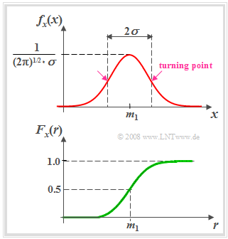
(1) »Probability density function« $($axisymmetric around $m_X)$
- $$f_X(x) = \frac{1}{\sqrt{2\pi}\cdot\sigma_X}\cdot {\rm e}^{-(X-m_X)^2 /(2\sigma_X^2) }.$$
PDF parameters:
- $m_X$ (mean or DC component),
- $σ_X$ (standard deviation or rms value).
(2) »Cumulative distribution function« $($point symmetric around $m_X)$
- $$F_X(x)= \phi(\frac{\it x-m_X}{\sigma_X})\hspace{0.5cm}\rm with\hspace{0.5cm}\rm \phi (\it x\rm ) = \frac{\rm 1}{\sqrt{\rm 2\it \pi}}\int_{-\rm\infty}^{\it x} \rm e^{\it -u^{\rm 2}/\rm 2}\,\, d \it u.$$
$ϕ(x)$: Gaussian error integral (cannot be calculated analytically, must be taken from tables).
(3) »Central moments«
- $$\mu_{k}=(k- 1)\cdot (k- 3) \ \cdots \ 3\cdot 1\cdot\sigma_X^k\hspace{0.2cm}\rm (if\hspace{0.2cm}\it k\hspace{0.2cm}\rm even).$$
- Charlier's skewness $S_X = 0$, since $\mu_3 = 0$ $($PDF is symmetric about $m_X)$.
- Kurtosis $K_X = 3$, since $\mu_4 = 3 \cdot \sigma_X^2$ ⇒ $K_X = 3$ results only for the Gaussian PDF.
(4) »Further remarks«
- The naming is due to the important mathematician, physicist and astronomer Carl Friedrich Gauss.
- If $m_X = 0$ and $σ_X = 1$, it is often referred to as the normal distribution.
- The standard deviation can also be determined graphically from the bell-shaped PDF $f_{X}(x)$ (as the distance between the maximum value and the point of inflection).
- Random quantities with Gaussian WDF are realistic models for many physical physical quantities and also of great importance for communications engineering.
- The sum of many small and independent components always leads to the Gaussian PDF ⇒ Central Limit Theorem of Statistics ⇒ Basis for noise processes.
- If one applies a Gaussian distributed signal to a linear filter for spectral shaping, the output signal is also Gaussian distributed.
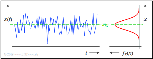
$\text{Example 1:}$ The graphic shows a section of a stochastic noise signal $x(t)$ whose instantaneous value can be taken as a continuous random variable $X$. From the PDF shown on the right, it can be seen that:
- A Gaussian random variable is present.
- Instantaneous values around the mean $m_X$ occur most frequently.
- If there are no statistical ties between the samples $x_ν$ of the sequence, such a signal is also called "white noise".
Uniformly distributed random variables
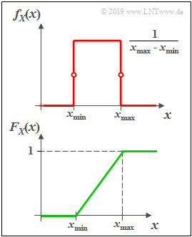
(1) »Probability density function«
- The probability density function (PDF) $f_{X}(x)$ is in the range from $x_{\rm min}$ to $x_{\rm max}$ constant equal to $1/(x_{\rm max} - x_{\rm min})$ and outside zero.
- At the range limits for $f_{X}(x)$ only half the value (mean value between left and right limit value) is to be set.
(2) »Cumulative distribution function«
- The cumulative distribution function (CDF) increases in the range from $x_{\rm min}$ to $x_{\rm max}$ linearly from zero to $1$.
'(3) »'«
- Mean and standard deviation have the following values for the uniform distribution:
- $$m_X = \frac{\it x_ {\rm max} \rm + \it x_{\rm min}}{2},\hspace{0.5cm} \sigma_X^2 = \frac{(\it x_{\rm max} - \it x_{\rm min}\rm )^2}{12}.$$
- For symmetric PDF ⇒ $x_{\rm min} = -x_{\rm max}$ the mean value $m_X = 0$ and the variance $σ_X^2 = x_{\rm max}^2/3.$
- Because of the symmetry around the mean $m_X$ the Charlier skewness $S_X = 0$.
- The kurtosis is with $K_X = 1.8$ significantly smaller than for the Gaussian distribution because of the absence of PDF outliers.
(4) »Further remarks«
- For modeling transmission systems, uniformly distributed random variables are the exception. An example of an actual (nearly) uniformly distributed random variable is the phase in circularly symmetric interference, such as occurs in quadrature amplitude modulation (QAM) schemes.
- The importance of uniformly distributed random variables for information and communication technology lies rather in the fact that, from the point of view of information theory, this PDF form represents an optimum with respect to differential entropy under the constraint of "peak limitation".
- In image processing & encoding, the uniform distribution is often used instead of the actual distribution of the original image, which is usually much more complicated, because the difference in information content between a natural image and the model based on the uniform distribution is relatively small.
- In the simulation of intelligence systems, one often uses "pseudo-random generators" based on the uniform distribution (which are relatively easy to realize), from which other distributions (Gaussian distribution, exponential distribution, etc.) can be easily derived.
Exponentially distributed random variables
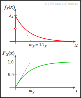
(1) »Probability distribution function«
An exponentially distributed random variable $X$ can only take on non–negative values. For $x>0$ the PDF has the following shape:
- $$f_X(x)=\it \lambda_X\cdot\rm e^{\it -\lambda_X \hspace{0.05cm}\cdot \hspace{0.03cm} x}.$$
- The larger the distribution parameter $λ_X$, the steeper the drop.
- By definition, $f_{X}(0) = λ_X/2$, which is the average of the left-hand limit $(0)$ and the right-hand limit $(\lambda_X)$.
(2) »Cumulative distribution function«
Distribution function PDF, we obtain for $x > 0$:
- $$F_{X}(x)=1-\rm e^{\it -\lambda_X\hspace{0.05cm}\cdot \hspace{0.03cm} x}.$$
(3) »Moments and central moments«
- The moments of the (one-sided) exponential distribution are generally equal to:
- $$m_k = \int_{-\infty}^{+\infty} x^k \cdot f_{X}(x) \,\,{\rm d} x = \frac{k!}{\lambda_X^k}.$$
- From this and from Steiner's theorem we get for mean and standard deviation:
- $$m_X = m_1=\frac{1}{\lambda_X},\hspace{0.6cm}\sigma_X^2={m_2-m_1^2}={\frac{2}{\lambda_X^2}-\frac{1}{\lambda_X^2}}=\frac{1}{\lambda_X^2}.$$
- The PDF is clearly asymmetric here. For the Charlier skewness $S_X = 2$.
- The kurtosis with $K_X = 9$ is clearly larger than for the Gaussian distribution, because the PDF foothills extend much further.
(4) »Further remarks«
- The exponential distribution has great importance for reliability studies; in this context, the term "lifetime distribution" is also commonly used.
- In these applications, the random variable is often the time $t$, that elapses before a component fails.
- Furthermore, it should be noted that the exponential distribution is closely related to the Laplace distribution.
Laplace distributed random variables
(1) »Probability density function«
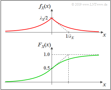
As can be seen from the graph, the Laplace distribution is a "two-sided exponential distribution":
- $$f_{X}(x)=\frac{\lambda_X} {2}\cdot{\rm e}^ { - \lambda_X \hspace{0.05cm} \cdot \hspace{0.05cm} \vert \hspace{0.05cm} x \hspace{0.05cm} \vert}.$$
- The maximum value here is $\lambda_X/2$.
- The tangent at $x=0$ intersects the abscissa at $1/\lambda_X$, as in the exponential distribution.
(2) »Cumulative distribution function«
- $$F_{X}(x) = {\rm Pr}\big [X \le x \big ] = \int_{-\infty}^{x} f_{X}(\xi) \,\,{\rm d}\xi $$
- $$\Rightarrow \hspace{0.5cm} F_{X}(x) = 0.5 + 0.5 \cdot {\rm sign}(x) \cdot \big [ 1 - {\rm e}^ { - \lambda_X \hspace{0.05cm} \cdot \hspace{0.05cm} \vert \hspace{0.05cm} x \hspace{0.05cm} \vert}\big ] $$
- $$\Rightarrow \hspace{0.5cm} F_{X}(-\infty) = 0, \hspace{0.5cm}F_{X}(0) = 0.5, \hspace{0.5cm} F_{X}(+\infty) = 1.$$
(3) »Moments and central moments«
- For odd $k$, the Laplace distribution always gives $m_k= 0$ due to symmetry. Among others: Linear mean $m_X =m_1 = 0$.
- For even $k$ the moments of Laplace distribution and exponential distribution agree: $m_k = {k!}/{\lambda^k}$.
- For the variance $(=$ second order central moment $=$ second order moment$)$ holds: $\sigma_X^2 = {2}/{\lambda_X^2}$ ⇒ twice as large as for the exponential distribution.
- For the Charlier skewness, $S_X = 0$ is obtained here due to the symmetric PDF.
- The kurtosis is $K_X = 6$, significantly larger than for the Gaussian distribution, but smaller than for the exponential distribution.
(4) »Further remarks«
- The instantaneous values of speech and music signals are Laplace distributed with good approximation.
See learning video "Wahrscheinlichkeit und Wahrscheinlichkeitsdichtefunktion", part 2. - By adding a Dirac delta function at $x=0$, speech pauses can also be modeled.
Brief description of other distributions
$\text{(A) Rayleigh distribution}$ $\text{More detailed description}$
- Probability density function:
- $$f_X(x) = \left\{ \begin{array}{c} x/\lambda_X^2 \cdot {\rm e}^{- x^2/(2 \hspace{0.05cm}\cdot\hspace{0.05cm} \lambda_X^2)} \\ 0 \end{array} \right.\hspace{0.15cm} \begin{array}{*{1}c} {\rm for}\hspace{0.1cm} x\hspace{-0.05cm} \ge \hspace{-0.05cm}0, \\ {\rm for}\hspace{0.1cm} x \hspace{-0.05cm}<\hspace{-0.05cm} 0. \\ \end{array}.$$
- Application: Modeling of the cellular channel (non-frequency selective fading, attenuation, diffraction, and refraction effects only, no line-of-sight).
$\text{(B) Rice distribution}$ $\text{More detailed description}$
- Probability density function $(\rm I_0$ denotes the modified zero-order Bessel function$)$:
- $$f_X(x) = \frac{x}{\lambda_X^2} \cdot {\rm exp} \big [ -\frac{x^2 + C_X^2}{2\cdot \lambda_X^2}\big ] \cdot {\rm I}_0 \left [ \frac{x \cdot C_X}{\lambda_X^2} \right ]\hspace{0.5cm}\text{with}\hspace{0.5cm}{\rm I }_0 (u) = {\rm J }_0 ({\rm j} \cdot u) = \sum_{k = 0}^{\infty} \frac{ (u/2)^{2k}}{k! \cdot \Gamma (k+1)} \hspace{0.05cm}.$$
- Application: Cellular channel modeling (non-frequency selective fading, attenuation, diffraction, and refraction effects only, with line-of-sight).
$\text{(C) Weibull distribution}$ $\text{More detailed description}$
- Probability density function:
- $$f_X(x) = \lambda_X \cdot k_X \cdot (\lambda_X \cdot x)^{k_X-1} \cdot {\rm e}^{(\lambda_X \cdot x)^{k_X}} \hspace{0.05cm}.$$
- Application: PDF with adjustable skewness $S_X$; exponential distribution $(k_X = 1)$ and Rayleigh distribution $(k_X = 2)$ included as special cases.
$\text{(D) Wigner semicircle distribution}$ $\text{More detailed description}$
- Probability density function:
- $$f_X(x) = \left\{ \begin{array}{c} 2/(\pi \cdot {R_X}^2) \cdot \sqrt{{R_X}^2 - (x- m_X)^2} \\ 0 \end{array} \right.\hspace{0.15cm} \begin{array}{*{1}c} {\rm for}\hspace{0.1cm} |x- m_X|\hspace{-0.05cm} \le \hspace{-0.05cm}R_X, \\ {\rm for}\hspace{0.1cm} |x- m_X| \hspace{-0.05cm} > \hspace{-0.05cm} R_X \\ \end{array}.$$
- Application: PDF of Chebyshev nodes ⇒ zeros of Chebyshev polynomials from numerics.
$\text{(E) Wigner parabolic distribution}$
- Probability density function:
- $$f_X(x) = \left\{ \begin{array}{c} 3/(4 \cdot {R_X}^3) \cdot \big ({R_X}^2 - (x- m_X)^2\big ) \\ 0 \end{array} \right.\hspace{0.15cm} \begin{array}{*{1}c} {\rm for}\hspace{0.1cm} |x|\hspace{-0.05cm} \le \hspace{-0.05cm}R_X, \\ {\rm for}\hspace{0.1cm} |x| \hspace{-0.05cm} > \hspace{-0.05cm} R_X \\ \end{array}.$$
- Application: PDF of eigenvalues of symmetric random matrices whose dimension approaches infinity.
$\text{(F) Cauchy distribution}$ $\text{More detailed description}$
- Probability density function and distribution function:
- $$f_{X}(x)=\frac{1}{\pi}\cdot\frac{\lambda_X}{\lambda_X^2+x^2}, \hspace{2cm} F_{X}(x)={\rm 1}/{2}+{\rm arctan}({x}/{\lambda_X}).$$
- In the Cauchy distribution, all moments $m_k$ for even $k$ have an infinitely large value, independent of the parameter $λ_X$.
- Thus, this distribution also has an infinitely large variance: $\sigma_X^2 \to \infty$.
- Due to symmetry, for odd $k$ all moments $m_k = 0$, if one assumes the "Cauchy Principal Value" as in the program: $m_X = 0, \ S_X = 0$.
- Example: The quotient of two Gaussian mean-free random variables is Cauchy distributed. For practical applications the Cauchy distribution has less meaning.
Exercises
- First, select the number $(1,\ 2, \text{...} \ )$ of the task to be processed. The number "$0$" corresponds to a "Reset": Same setting as at program start.
- A task description is displayed. The parameter values are adjusted. Solution after pressing "Show Solution".
- In the following $\text{Red}$ stands for the random variable $X$ and $\text{Blue}$ for $Y$.
(1) Select $\text{red: Gaussian PDF}\ (m_X = 1, \ \sigma_X = 0.4)$ and $\text{blue: Rectangular PDF}\ (y_{\rm min} = -2, \ y_{\rm max} = +3)$. Interpret the $\rm PDF$ graph.
- $\text{Gaussian PDF}$: The $\rm PDF$ maximum is equal to $f_{X}(x = m_X) = \sqrt{1/(2\pi \cdot \sigma_X^2)} = 0.9974 \approx 1$.
- $\text{Rectangular PDF}$: All $\rm PDF$ values are equal $0.2$ in the range $-2 < y < +3$. At the edges $f_Y(-2) = f_Y(+3)= 0.1$ (half value) holds.
(2) Same setting as for $(1)$. What are the probabilities ${\rm Pr}(X = 0)$, ${\rm Pr}(0.5 \le X \le 1.5)$, ${\rm Pr}(Y = 0)$ and ${\rm Pr}(0.5 \le Y \le 1.5)$ .
- ${\rm Pr}(X = 0)={\rm Pr}(Y = 0) \equiv 0$ ⇒ Probability of a discrete random variable to take exactly a certain value.
- The other two probabilities can be obtained by integration over the PDF in the range $+0.5\ \text{...} \ +\hspace{-0.1cm}1.5$.
- Or: ${\rm Pr}(0.5 \le X \le 1.5)= F_X(1.5) - F_X(0.5) = 0.8944-0.1056 = 0.7888$. Correspondingly: ${\rm Pr}(0.5 \le Y \le 1.5)= 0.7-0.5=0.2$.
(3) Same settings as before. How must the standard deviation $\sigma_X$ be changed so that with the same mean $m_X$ it holds for the second order moment: $P_X=2$ ?
- According to Steiner's theorem: $P_X=m_X^2 + \sigma_X^2$ ⇒ $\sigma_X^2 = P_X-m_X^2 = 2 - 1^2 = 1 $ ⇒ $\sigma_X = 1$.
(4) Same settings as before: How must the parameters $y_{\rm min}$ and $y_{\rm max}$ of the rectangular PDF be changed to yield $m_Y = 0$ and $\sigma_Y^2 = 0.75$?
- Starting from the previous setting $(y_{\rm min} = -2, \ y_{\rm max} = +3)$ we change $y_{\rm max}$ until $\sigma_Y^2 = 0.75$ occurs ⇒ $y_{\rm max} = 1$.
- The width of the rectangle is now $3$. The desired mean $m_Y = 0$ is obtained by shifting: $y_{\rm min} = -1.5, \ y_{\rm max} = +1.5$.
- You could also consider that for a mean-free random variable $(y_{\rm min} = -y_{\rm max})$ the following equation holds: $\sigma_Y^2 = y_{\rm max}^2/3$.
(5) For which of the adjustable distributions is the Charlier skewness $S \ne 0$ ?
- The Charlier's skewness denotes the third central moment related to $σ_X^3$ ⇒ $S_X = \mu_3/σ_X^3$ $($valid for the random variable $X)$.
- If the PDF $f_X(x)$ is symmetric around the mean $m_X$ then the parameter $S_X$ is always zero.
- Exponential distribution: $S_X =2$; Rayleigh distribution: $S_X =0.631$ $($both independent of $λ_X)$; Rice distribution: $S_X >0$ $($dependent of $C_X, \ λ_X)$.
- With the Weibull distribution, the Charlier skewness $S_X$ can be zero, positive or negative, depending on the PDF parameter $k_X$.
- Weibull distribution, $\lambda_X=0.4$: With $k_X = 1.5$ ⇒ PDF is curved to the left $(S_X > 0)$; $k_X = 7$ ⇒ PDF is curved to the right $(S_X < 0)$.
(6) Select $\text{Red: Gaussian PDF}\ (m_X = 1, \ \sigma_X = 0.4)$ and $\text{Blue: Gaussian PDF}\ (m_X = 0, \ \sigma_X = 1)$. What is the kurtosis in each case?
- For each Gaussian distribution the kurtosis has the same value: $K_X = K_Y =3$. Therefore, $K-3$ is called "excess".
- This parameter can be used to check whether a given random variable can be approximated by a Gaussian distribution.
(7) For which distributions does a significantly smaller kurtosis value result than $K=3$? And for which distributions does a significantly larger one?
- $K<3$ always results when the PDF values are more concentrated around the mean than in the Gaussian distribution.
- This is true, for example, for the uniform distribution $(K=1.8)$ and for the triangular distribution $(K=2.4)$.
- $K>3$, if the PDF offshoots are more pronounced than for the Gaussian distribution. Example: Exponential PDF $(K=9)$.
(8) Select $\text{Red: Exponential PDF}\ (\lambda_X = 1)$ and $\text{Blue: Laplace PDF}\ (\lambda_Y = 1)$. Interpret the differences.
- The Laplace distribution is symmetric around its mean $(S_Y=0, \ m_Y=0)$ unlike the exponential distribution $(S_X=2, \ m_X=1)$.
- The even moments $m_2, \ m_4, \ \text{...}$ are equal, for example: $P_X=P_Y=2$. But not the variances: $\sigma_X^2 =1, \ \sigma_Y^2 =2$.
- The probabilities ${\rm Pr}(|X| < 2) = F_X(2) = 0.864$ and ${\rm Pr}(|Y| < 2) = F_Y(2) - F_Y(-2)= 0.932 - 0.068 = 0.864$ are equal.
- In the Laplace PDF, the values are more tightly concentrated around the mean than in the exponential PDF: $K_Y =6 < K_X = 9$.
(9) Select $\text{Red: Rice PDF}\ (\lambda_X = 1, \ C_X = 1)$ and $\text{Blue: Rayleigh PDF}\ (\lambda_Y = 1)$. Interpret the differences.
- With $C_X = 0$ the Rice PDF transitions to the Rayleigh PDF. A larger $C_X$ improves the performance, e.g., in mobile communications.
- Both, in "Rayleigh" and "Rice" the abscissa is the magnitude $A$ of the received signal. Favorably, if ${\rm Pr}(A \le A_0)$ is small $(A_0$ given$)$.
- For $C_X \ne 0$ and equal $\lambda$ the Rice CDF is below the Rayleigh CDF ⇒ smaller ${\rm Pr}(A \le A_0)$ for all $A_0$.
(10) Select $\text{Red: Rice PDF}\ (\lambda_X = 0.6, \ C_X = 2)$. By which distribution $F_Y(y)$ can this Rice distribution be well approximated?
- The kurtosis $K_X = 2.9539 \approx 3$ indicates the Gaussian distribution. Favorable parameters: $m_Y = 2.1 > C_X, \ \ \sigma_Y = \lambda_X = 0.6$.
- The larger tht quotient $C_X/\lambda_X$ is, the better the Rice PDF is approximated by a Gaussian PDF.
- For large $C_X/\lambda_X$ the Rice PDF has no more similarity with the Rayleigh PDF.
(11) Select $\text{Red: Weibull PDF}\ (\lambda_X = 1, \ k_X = 1)$ and $\text{Blue: Weibull PDF}\ (\lambda_Y = 1, \ k_Y = 2)$. Interpret the results.
- The Weibull PDF $f_X(x)$ is identical to the exponential PDF and $f_Y(y)$ to the Rayleigh PDF.
- However, after best fit, the parameters $\lambda_{\rm Weibull} = 1$ and $\lambda_{\rm Rayleigh} = 0.7$ differ.
- Moreover, it holds $f_X(x = 0) \to \infty$ for $k_X < 1$. However, this does not have the affect of infinite moments.
(12) Select $\text{Red: Weibull PDF}\ (\lambda_X = 1, \ k_X = 1.6)$ and $\text{Blue: Weibull PDF}\ (\lambda_Y = 1, \ k_Y = 5.6)$. Interpret the Charlier skewness.
- One observes: For the PDF parameter $k < k_*$ the Charlier skewness is positive and for $k > k_*$ negative. It is approximately $k_* = 3.6$.
(13) Select $\text{Red: Semicircle PDF}\ (m_X = 0, \ R_X = 1)$ and $\text{Blue: Parabolic PDF}\ (m_Y = 0, \ R_Y = 1)$. Vary the parameter $R$ in each case.
- The PDF in each case is mean-free and symmetric $(S_X = S_Y =0)$ with $\sigma_X^2 = 0.25, \ K_X = 2$ respectively, $\sigma_Y^2 = 0.2, \ K_Y \approx 2.2$.
Applet Manual
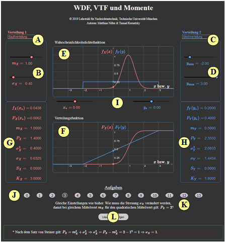
(A) Selection of the distribution $f_X(x)$ (red curves and output values)
(B) Parameter input for the "red distribution" via slider
(C) Selection of the distribution $f_Y(y)$ (blue curves and output values)
(D) Parameter input for the "red distribution" via slider
(E) Graphic area for the probability density function (PDF)
(F) Graphic area for the distribution function (CDF)
(G) Numerical output for the "red distribution"
(H) Numerical output for the "blue distribution"
( I ) Input of $x_*$ and $y_*$ abscissa values for the numerics outputs
(J) Experiment execution area: task selection
(K) Experiment execution area: task description
( L) Experiment execution area: sample solution
Selection options for for $\rm A$ and $\rm C$:
Gaussian distribution, uniform distribution, triangular distribution, exponential distribution, Laplace distribution, Rayleigh distribution, Rice distribution, Weibull distribution, Wigner semicircle distribution, Wigner parabolic distribution, Cauchy distribution.
The following »integral parameters« are output $($with respect to $X)$:
Linear mean value $m_X = {\rm E}\big[X \big]$, second order moment $P_X ={\rm E}\big[X^2 \big] $, variance $\sigma_X^2 = P_X - m_X^2$, standard deviation $\sigma_X$, Charlier's skewness $S_X$, kurtosis $K_X$.
In all applets top right: Changeable graphical interface design ⇒ Theme:
- Dark: black background (recommended by the authors).
- Bright: white background (recommended for beamers and printouts)
- Deuteranopia: for users with pronounced green–visual impairment
- Protanopia: for users with pronounced red–visual impairment
About the Authors
This interactive calculation tool was designed and implemented at the $\text{Institute for Communications Engineering}$ at the $\text{Technical University of Munich}$.
- The first version was created in 2005 by »Bettina Hirner« as part of her diploma thesis with “FlashMX – Actionscript” (Supervisor: »Günter Söder« and »Klaus Eichin« ).
- In 2019 the program was redesigned via HTML5/JavaScript by »Matthias Niller« (Ingenieurspraxis Mathematik, Supervisor: »Benedikt Leible« and »Tasnád Kernetzky« ).
- Last revision and English version 2021 by »Carolin Mirschina« in the context of a working student activity.
- The conversion of this applet was financially supported by $\text{Studienzuschüsse}$ (TUM Department of Electrical and Computer Engineering). We thank.
