Difference between revisions of "Examples of Communication Systems/Speech Coding"
| Line 160: | Line 160: | ||
<br clear=all> | <br clear=all> | ||
It should be noted with regard to this block diagram: | It should be noted with regard to this block diagram: | ||
| − | *RPE coding is performed for $5 \rm ms$ subframes $(40$ samples$)$ respectively. This is indicated here by the index $i$ in the input signal $e_{\rm LTP},\hspace{0.03cm} i(l)$ where with $i = 1, 2, 3, 4$ again the individual | + | *RPE coding is performed for $5 \rm ms$ subframes $(40$ samples$)$ respectively. This is indicated here by the index $i$ in the input signal $e_{\rm LTP},\hspace{0.03cm} i(l)$ where with $i = 1, 2, 3, 4$ again the individual subblocks are numbered. |
*In the first step, the LTP prediction error signal $e_{{\rm LTP}, \hspace{0.03cm}i}(l)$ is bandlimited by a low-pass filter to about one third of the original bandwidth - i.e. to $1.3 \rm kHz$ . In a second step, this enables a reduction of the sampling rate by a factor of about $3$. | *In the first step, the LTP prediction error signal $e_{{\rm LTP}, \hspace{0.03cm}i}(l)$ is bandlimited by a low-pass filter to about one third of the original bandwidth - i.e. to $1.3 \rm kHz$ . In a second step, this enables a reduction of the sampling rate by a factor of about $3$. | ||
*So the output signal $x_i(l)$ with $l = 1$, ... , $40$ by subsampling into four subsequences $x_{m, \hspace{0.03cm} i}(j)$ with $m = 1$, ... , $4$ and $j = 1$, ... , $13$ decomposed. This decomposition is illustrated in the diagram. | *So the output signal $x_i(l)$ with $l = 1$, ... , $40$ by subsampling into four subsequences $x_{m, \hspace{0.03cm} i}(j)$ with $m = 1$, ... , $4$ and $j = 1$, ... , $13$ decomposed. This decomposition is illustrated in the diagram. | ||
| Line 173: | Line 173: | ||
*From the optimal subsequence for the subblock $i$ $($with index $M_i)$ the ''amplitude maximum'' $x_{\rm max,\hspace{0.03cm}i}$ is determined, this value is logarithmically quantised with six bits and made available for transmission as $\mathbf{x_{\rm max}}(i)$ . In total, the four RPE block amplitudes require $24$ bits. | *From the optimal subsequence for the subblock $i$ $($with index $M_i)$ the ''amplitude maximum'' $x_{\rm max,\hspace{0.03cm}i}$ is determined, this value is logarithmically quantised with six bits and made available for transmission as $\mathbf{x_{\rm max}}(i)$ . In total, the four RPE block amplitudes require $24$ bits. | ||
*In addition, for each subblock $i$ the optimal subsequence is normalised to $x_{{\rm max},\hspace{0.03cm}i}$ . The obtained $13$ samples are then quantised with three bits each and transmitted encoded as $\mathbf{X}_j(i)$ . The $4 - 13 - 3 = 156$ bits describe the so-called '''RPE pulse'''. | *In addition, for each subblock $i$ the optimal subsequence is normalised to $x_{{\rm max},\hspace{0.03cm}i}$ . The obtained $13$ samples are then quantised with three bits each and transmitted encoded as $\mathbf{X}_j(i)$ . The $4 - 13 - 3 = 156$ bits describe the so-called '''RPE pulse'''. | ||
| − | *Then these RPE parameters are decoded locally again and fed back as a signal $e_{{\rm RPE},\hspace{0.03cm}i}(l)$ to the LTP synthesis filter in the previous | + | *Then these RPE parameters are decoded locally again and fed back as a signal $e_{{\rm RPE},\hspace{0.03cm}i}(l)$ to the LTP synthesis filter in the previous subblock, from which, together with the LTP estimation signal $y_i(l)$ the signal $e\hspace{0.03cm}'_i(l)$ is generated (see [[Examples_of_Communication_Systems/Voice_Coding#Long_Term_Prediction|"LTP–Graph"]]). |
*By interposing two zero values between each two transmitted RPE samples, the baseband from zero to $1300 \ \rm Hz$ in the range from $1300 \ \rm Hz$ to $2600 \ \ \rm Hz$ in sweep position and from $2600 \ \ \rm Hz$ to $3900 \ \rm Hz$ in normal position. This is the reason for the necessary DC signal release in the preprocessing. Otherwise, a disturbing whistling tone at $2.6 \ \rm kHz$ would result from the described convolution operation. | *By interposing two zero values between each two transmitted RPE samples, the baseband from zero to $1300 \ \rm Hz$ in the range from $1300 \ \rm Hz$ to $2600 \ \ \rm Hz$ in sweep position and from $2600 \ \ \rm Hz$ to $3900 \ \rm Hz$ in normal position. This is the reason for the necessary DC signal release in the preprocessing. Otherwise, a disturbing whistling tone at $2.6 \ \rm kHz$ would result from the described convolution operation. | ||
| Line 208: | Line 208: | ||
The following descriptions mostly refer to the mode with $12.2 \ \rm kbit/s$. | The following descriptions mostly refer to the mode with $12.2 \ \rm kbit/s$. | ||
| − | [[File:EN | + | [[File:EN Bei T 3 3 S8c.png|right|frame|Compilation of AMR parameters]] |
*All predecessor methods of the AMR are based on minimising the prediction error signal by forward prediction in the substeps LPC, LTP and RPE. | *All predecessor methods of the AMR are based on minimising the prediction error signal by forward prediction in the substeps LPC, LTP and RPE. | ||
| Line 224: | Line 224: | ||
[[File:EN_Bei_T_3_3_S8.png|center|frame|Algebraic Code Excited Linear Prediction – Principle]] | [[File:EN_Bei_T_3_3_S8.png|center|frame|Algebraic Code Excited Linear Prediction – Principle]] | ||
| − | * | + | *The voice signal $s(n)$, sampled at $8 \ \rm kHz$ and quantised at $13$ bit, as in the GSM fullrate speech codec, is divided into frames $s_{\rm R}(n)$ with $n = 1$, ..., before further processing. , $160$ or into subblocks $s_i(l)$ with $i = 1, 2, 3, 4$ and $l = 1$, ... , $40$ segmented. |
| − | * | + | *The calculation of the LPC coefficients is done in the red highlighted block frame by frame every $20 \ \rm ms$ corresponding to $160$ samples, since within this short time span the spectral envelope of the speech signal $s_{\rm R}(n)$ can be considered constant. |
| − | * | + | *For LPC analysis, a filter $A(z)$ of order $10$ is usually chosen. In the highest-rate mode with $12.2 \ \rm kbit/s$ the current coefficients $a_k \ ( k = 1$, ... , $10)$ of the short-time prediction are quantised every $10\ \rm ms$ , coded and made available for transmission at the point '''1''' highlighted in yellow. |
| − | * | + | *The further steps of the AMR are carried out every $5 \ \rm ms$ according to the $40$ samples of the signals $s_i(l)$ . The long-term prediction (LTP) - outlined in blue in the picture - is realised here as an adaptive codebook in which the samples of the preceding subblocks are entered. |
| − | * | + | *For the long-term prediction (LTP), first the gain $G_{\rm FCB}$ for the ''Fixed Code Book'' (FCB) is set to zero, so that a sequence of $40$ samples of the adaptive code book are present at the input $u_i(l)$ of the speech tract filter set by the LPC $A(z)^{-1}$ . The index $i$ denotes the subblock under consideration. |
| − | * | + | *By varying the two LTP parameters $N_{{\rm LTP},\hspace{0.05cm}i}$ and $G_{{\rm LTP},\hspace{0.05cm}i}$ shall be achieved for this $i$-th subblock that the root mean square - i.e. the mean power - of the weighted error signal $w_i(l)$ becomes minimal. |
| − | * | + | *The error signal $w_i(l)$ is equal to the difference between the current speech frame $s_i(l)$ and the output signal $y_i(l)$ of the so-called speech tract filter when excited with $u_i(l)$, taking into account the weighting filter $W(z)$ to match the spectral characteristics of human hearing. |
| − | *In | + | *In other words, $W(z)$ removes those spectral components in the signal $e_i(l)$ that are not perceived by an "average" ear. In the mode $12.2 \ \rm kbit/s$ one uses $W(z) = A(z/γ_1)/A(z/γ_2)$ with constant factors $γ_1 = 0.9$ and $γ_2 = 0.6$. |
| − | * | + | *For each subblock, denotes $N_{{\rm LTP},\hspace{0.05cm}i}$ the best possible LTP delay, which together with the LTP gain $G_{{\rm LTP},\hspace{0.05cm}i}$ after averaging with respect to $l = 1$, ... , $40$ minimises the squared error $\text{E}[w_i(l)^2]$ . Dashed lines indicate control lines for iterative optimisation. |
| − | * | + | *The procedure described is called '''analysis by synthesis'''. After a sufficiently large number of iterations, the subblock $u_i(l)$ is included in the adaptive codebook. The determined LTP parameters $N_{{\rm LTP},\hspace{0.05cm}i}$ and $G_{{\rm LTP},\hspace{0.05cm}i}$ are encoded and made available for transmission. |
Revision as of 20:43, 21 January 2023
Contents
- 1 Various voice coding methods
- 2 GSM Fullrate Vocoder
- 3 Linear Predictive Coding
- 4 Long Term Prediction
- 5 Regular Pulse Excitation – RPE Coding
- 6 Halfrate Vocoder and Enhanced Fullrate Codec
- 7 Adaptive Multi–Rate Codec
- 8 Algebraic Code Excited Linear Prediction
- 9 Fixed Code Book – FCB
- 10 Aufgaben zum Kapitel
- 11 References
Various voice coding methods
Each GSM subscriber has a maximum net data rate of $\text{22.8 kbit/s}$ available, while the ISDN fixed network operates with a data rate of $\text{64 kbit/s}$ $($with $8$ bit quantization$)$ or $\text{104 kbit/s}$ $($with $13$ bit quantization$)$ respectively.
- The task of "voice coding" $($"speech coding"$)$ in GSM is to limit the amount of data for speech signal transmission to $\text{22.8 kbit/s}$ and to reproduce the speech signal at the receiver side in the best possible way.
- The functions of the GSM encoder and the GSM decoder are usually combined in a single functional unit called "codec".
Different signal processing methods are used for voice coding and decoding:
- The GSM Fullrate Vocoder was standardized in 1991 from a combination of three compression methods for the GSM radio channel. It is based on "Linear Predictive Coding" $\rm (LPC)$ in conjunction with "Long Term Prediction" $\rm (LTP)$ and "Regular Pulse Excitation" $\rm (RPE)$.
- The GSM Halfrate Vocoder was introduced in 1994 and provides the ability to transmit speech at nearly the same quality in half a traffic channel $($data rate $\text{11.4 kbit/s})$.
- The Enhanced Full Rate Vocoder $\rm (EFR\ codec)$ was standardized and implemented in 1995, originally for the North American DCS1900 network. The EFR codec provides better voice quality compared to the conventional full rate codec.
- The Adaptive Multi-Rate Codec $\rm (AMR\ codec)$ is the latest voice codec for GSM. It was standardized in 1997 and also mandated in 1999 by the "Third Generation Partnership Project" $\rm (3GPP)$ as the standard voice codec for third generation mobile systems such as UMTS.
- In contrast to conventional AMR, where the voice signal is bandlimited to the frequency range from $\text{300 Hz}$ to $\text{3.4 kHz}$, "'Wideband AMR", which was developed and standardized for UMTS in 2007, assumes a wideband signal $\text{(50 Hz - 7 kHz)}$. This is therefore also suitable for music signals.
⇒ You can visualize the quality of these voice coding schemes for speech and music with the $($German language$)$ SWF applet
"Qualität verschiedener Sprach–Codecs" ⇒ "Quality of different voice codecs".
GSM Fullrate Vocoder
In the »Full Rate Vocoder«, the analog speech signal in the frequency range between $300 \ \rm Hz$ and $3400 \ \rm Hz$
- is first sampled with $8 \ \rm kHz$ and
- then linearly quantized with $13$ bits ⇒ »A/D conversion«,
resulting in a data rate of $104 \ \rm kbit/s$.
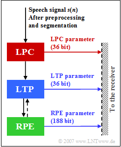
In this method, speech coding is performed in four steps:
- The preprocessing,
- the setting of the short-term analyze filter $($Linear Predictive Coding, $\rm LPC)$,
- the control of the Long Term Prediction $\rm (LTP)$ filter, and
- the encoding of the residual signal by a sequence of pulses $($Regular Pulse Excitation, $\rm RPE)$.
In the upper graph, $s(n)$ denotes the speech signal sampled and quantized at distance $T_{\rm A} = 125\ \rm µ s$ after the continuously performed preprocessing, where
- the digitized microphone signal is freed from a possibly existing DC signal component $($"offset"$)$ in order to avoid a disturbing whistling tone of approx. $2.6 \ \rm kHz$ during decoding when recovering the higher frequency components, and
- additionally, higher spectral components of $s(n)$ are raised to improve the computational accuracy and effectiveness of the subsequent LPC analysis.
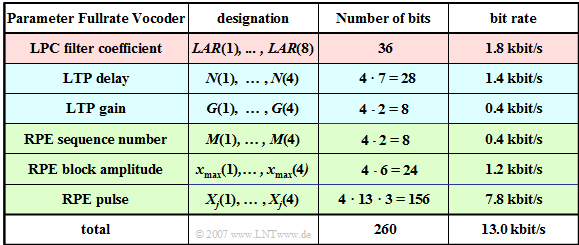
The table shows the $76$ parameters $(260$ bit$)$ of the functional units LPC, LTP and RPE. The meaning of the individual quantities is described in detail on the following pages.
All processing steps $($LPC, LTP, RPE$)$ are performed in blocks of $20 \ \rm ms$ duration over $160$ samples of the preprocessed speech signal, which are called »GSM speech frames« .
- In the full rate codec, a total of $260$ bits are generated per voice frame, resulting in a data rate of $13 \rm kbit/s$.
- This corresponds to a compression of the speech signal by a factor $8$ $(104 \ \rm kbit/s$ related to $13 \ \rm kbit/s)$.
Linear Predictive Coding
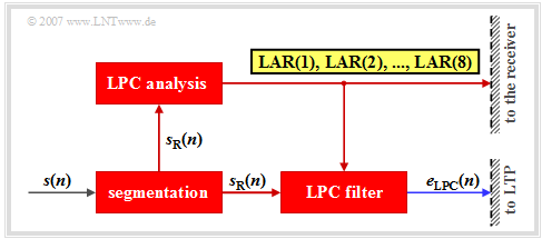
The block «Linear Predictive Coding» $\rm (LPC)$ performs short-time prediction, that is, it determines the statistical dependencies among the samples in a short range of one millisecond. The following is a brief description of the LPC principle circuit:
- First, for this purpose the time-unlimited signal $s(n)$ is segmented into intervals $s_{\rm R}(n)$ of $20\ \rm ms$ duration $(160$ samples$)$. By convention, the run variable within such a speech frame $($German: "Rahmen" ⇒ subscript: "R"$)$ can take the values $n = 1$, ... , $160$.
- In the first step of LPC analysis dependencies between samples are quantified by the autocorrelation $\rm ACF)$ coefficients with indices $0 ≤ k ≤ 8$ :
- $$φ_{\rm s}(k) = \text{E}\big [s_{\rm R}(n) · s_{\rm R}(n + k)\big ].$$
- From these nine ACF values, using the so-called "Schur recursion" eight reflection coefficients $r_{k}$ are calculated, which serve as a basis for setting the coefficients of the LPC analysis filter for the current frame.
- The coefficients $r_{k}$ have values between $±1$. Even small changes in $r_{k}$ at the edge of their value range cause large changes for speech coding. The eight reflectance values $r_{k}$ are represented logarithmically ⇒ LAR parameters $($"Log Area Ratio"$)$:
- $${\rm LAR}(k) = \ln \ \frac{1-r_k}{1+r_k}, \hspace{1cm} k = 1,\hspace{0.05cm} \text{...}\hspace{0.05cm} , 8.$$
- Then, the eight LAR parameters are quantized by different bit numbers according to their subjective meaning, encoded and made available for transmission.
- The first two parameters are represented with six bits each,
- the next two with five bits each,
- $\rm LAR(5)$ and $\rm LAR(6)$ with four bits each, and
- the last two – $\rm LAR(7)$ and $\rm LAR(8)$– with three bits each.
- If the transmission is error-free, the original speech signal $s(n)$ can be completely reconstructed again at the receiver from the eight LPC parameters $($in total $36$ bits$)$ with the corresponding LPC synthesis filter, if one disregards the unavoidable additional quantization errors due to the digital description of the LAR coefficients.
- Further, the prediction error signal $e_{\rm LPC}(n)$ is obtained using the LPC filter. This is also the input signal for the subsequent long-term prediction. The LPC filter is not recursive and has only a short memory of about one millisecond.
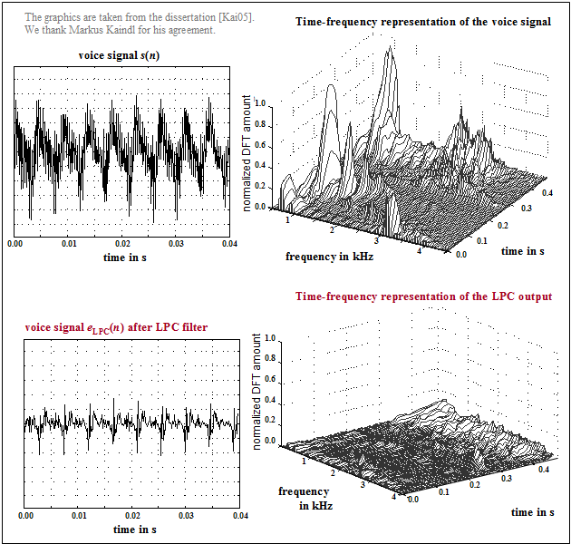
$\text{Example 1:}$ The graph from [Kai05][1] shows
- top left: a section of the speech signal $s(n)$,
- top right: its time-frequency representation,
- bottom left: the LPC prediction error signal $e_{\rm LPC}(n)$,
- bottom right: its time-frequency representation,
One can see from these pictures
- the smaller amplitude of $e_{\rm LPC}(n)$ compared to $s(n)$,
- the significantly reduced dynamic range, and
- the flatter spectrum of the remaining signal.
Long Term Prediction
Long Term Prediction (LTP) exploits the property of the speech signal that it also has periodic structures (voiced sections). This fact is used to reduce the redundancy present in the signal.
- The long-term prediction (LTP analysis and filtering) is performed four times per speech frame, i.e. every $5 \rm ms$ .
- The four subblocks consist of $40$ samples each and are identified by $i = 1$, ... , $4$ numbered.
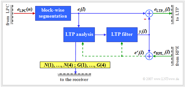
The following is a short description according to the above LTP–schematic diagram - see [Kai05][1].
- The input signal is the output signal $e_{\rm LPC}(n)$ of the short-term prediction. The signals after segmentation into four subblocks are denoted by $e_i(l)$ where each $l = 1, 2$, ... , $40$ holds.
- For this analysis, the cross-correlation function $φ_{ee\hspace{0.03cm}',\hspace{0.05cm}i}(k)$ of the current subblock $i$ of the LPC predictor error signal $e_i(l)$ with the reconstructed LPC residual signal $e\hspace{0.03cm}'_i(l)$ from the three previous subframes. The memory of this LTP predictor is between $5 \ \rm ms$ and $15 \ \rm ms$ and is thus significantly longer than that of the LPC predictor $(1 \ \rm ms)$.
- $e\hspace{0.03cm}'_i(l)$ is the sum of the LTP filter output signal $y_i(l)$ and the correction signal $e_{\rm RPE,\hspace{0.05cm}i}(l)$ provided by the following component (Regular Pulse Excitation) for the $i$-th subblock.
- The value of $k$ for which the cross-correlation function $φ_{ee\hspace{0.03cm}',\hspace{0.05cm}i}(k)$ becomes maximum determines the optimal LTP delay $N(i)$ for each subblock $i$ . The delays $N(1)$ to $N(4)$ are each quantised to seven bits and made available for transmission.
- The gain factor $G(i)$ associated with $N(i)$ - also called LTP gain - is determined so that the subblock found at the location $N(i)$ after multiplication by $G(i)$ best matches the current subframe $e_i(l)$ . The gains $G(1)$ to $G(4)$ are each quantised by two bits and together with $N(1)$, ..., $N(4)$ give the $36$ bits for the eight LTP parameters.
- The signal $y_i(l)$ after LTP analysis and filtering is an estimated signal for the LPC signal $e_i(l)$ in $i$-th subblock. The difference between the two gives the LTP residual signal $e_{\rm LTP,\hspace{0.05cm}i}(l)$, which is passed on to the next functional unit "RPE".
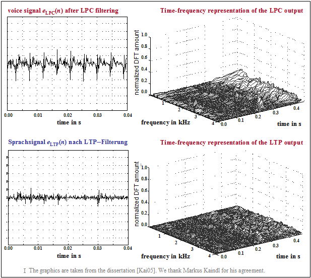
$\text{Example 2:}$ The graph from [Kai05][1] shows.
- above the LPC prediction error signal $e_{\rm LPC}(n)$ - simultaneously the LTP input signal,
- below the residual error signal $e_{\rm LTP}(n)$ after long-term prediction.
Only one subblock is considered. Therefore, the same letter $n$ is used here for the discrete time in LPC and LTP.
One can see from these representations
- the smaller amplitudes of $e_{\rm LTP}(n)$ compared to $e_{\rm LPC}(n)$ and
- the significantly reduced dynamic range of $e_{\rm LTP}(n)$,
- especially in periodic, i.e. voiced, sections.
Also in the frequency domain, a reduction of the prediction error signal due to the long-term prediction is evident.
Regular Pulse Excitation – RPE Coding
The signal after LPC and LTP filtering is already redundancy–reduced, i.e. it requires a lower bit rate than the sampled speech signal $s(n)$.
- Now, in the following functional unit Regular Pulse Excitation (RPE) the irrelevance is further reduced.
- This means that signal components that are less important for the subjective hearing impression are removed.
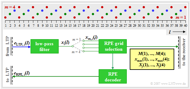
It should be noted with regard to this block diagram:
- RPE coding is performed for $5 \rm ms$ subframes $(40$ samples$)$ respectively. This is indicated here by the index $i$ in the input signal $e_{\rm LTP},\hspace{0.03cm} i(l)$ where with $i = 1, 2, 3, 4$ again the individual subblocks are numbered.
- In the first step, the LTP prediction error signal $e_{{\rm LTP}, \hspace{0.03cm}i}(l)$ is bandlimited by a low-pass filter to about one third of the original bandwidth - i.e. to $1.3 \rm kHz$ . In a second step, this enables a reduction of the sampling rate by a factor of about $3$.
- So the output signal $x_i(l)$ with $l = 1$, ... , $40$ by subsampling into four subsequences $x_{m, \hspace{0.03cm} i}(j)$ with $m = 1$, ... , $4$ and $j = 1$, ... , $13$ decomposed. This decomposition is illustrated in the diagram.
- The subsequences $x_{m,\hspace{0.03cm} i}(j)$ include the following samples of the signal $x_i(l)$:
- $m = 1$: $l = 1, \ 4, \ 7$, ... , $34, \ 37$ (red dots),
- $m = 2$: $l = 2, \ 5, \ 8$, ... , $35, \ 38$ (green dots),
- $m = 3$: $l = 3, \ 6, \ 9$, ... , $36, \ 39$ (blue dots),
- $m = 4$: $l = 4, \ 7, \ 10$, ... , $37, \ 40$ $($also red, largely identical to $m = 1)$.
- For each subblock $i$ in the block RPE Grid Selection the subsequence $x_{m,\hspace{0.03cm}i}(j)$ with the highest energy is selected and the index $M_i$ of the optimal sequence is quantised with two bits and transmitted as $\mathbf{M}(i)$ . In total, the four RPE subsequence indices require $\mathbf{M}(1)$, ... , $\mathbf{M}(4)$ thus eight bits.
- From the optimal subsequence for the subblock $i$ $($with index $M_i)$ the amplitude maximum $x_{\rm max,\hspace{0.03cm}i}$ is determined, this value is logarithmically quantised with six bits and made available for transmission as $\mathbf{x_{\rm max}}(i)$ . In total, the four RPE block amplitudes require $24$ bits.
- In addition, for each subblock $i$ the optimal subsequence is normalised to $x_{{\rm max},\hspace{0.03cm}i}$ . The obtained $13$ samples are then quantised with three bits each and transmitted encoded as $\mathbf{X}_j(i)$ . The $4 - 13 - 3 = 156$ bits describe the so-called RPE pulse.
- Then these RPE parameters are decoded locally again and fed back as a signal $e_{{\rm RPE},\hspace{0.03cm}i}(l)$ to the LTP synthesis filter in the previous subblock, from which, together with the LTP estimation signal $y_i(l)$ the signal $e\hspace{0.03cm}'_i(l)$ is generated (see "LTP–Graph").
- By interposing two zero values between each two transmitted RPE samples, the baseband from zero to $1300 \ \rm Hz$ in the range from $1300 \ \rm Hz$ to $2600 \ \ \rm Hz$ in sweep position and from $2600 \ \ \rm Hz$ to $3900 \ \rm Hz$ in normal position. This is the reason for the necessary DC signal release in the preprocessing. Otherwise, a disturbing whistling tone at $2.6 \ \rm kHz$ would result from the described convolution operation.
Halfrate Vocoder and Enhanced Fullrate Codec
After the standardisation of the fullrate codec in 1991, the subsequent focus was on the development of new speech codecs with two specific objectives, namely.
- the better utilisation of the bandwidth available in GSM systems, and
- the improvement of voice quality.
This development can be summarised as follows:
- By 1994, a new process was developed with the Halfrate Vocoder. This has a data rate of $5.6 kbit/s$ and thus offers the possibility of transmitting speech in half a traffic channel with approximately the same quality. This allows two calls to be handled simultaneously on one time slot. However, the half-rate codec was only used by mobile phone operators when a radio cell was congested. In the meantime, the half-rate codec no longer plays a role.
- In order to further improve the voice quality, the Enhanced Fullrate Codec (EFR codec) was introduced in 1995. This voice coding method - originally developed for the US DCS1900 network - is a full-rate codec with the (slightly lower) data rate $12.2 \ \rm kbit/s$. The use of this codec must of course be supported by the mobile phone.
- Instead of the RPE-LTP compression (Regular Pulse Excitation - Long Term Prediction) of the conventional full rate codec, this further development also uses Algebraic Code Excitation Linear Prediction (ACELP), which offers a significantly better speech quality and also improved error detection and concealment. More information about this can be found on the next page but one.
Adaptive Multi–Rate Codec
The GSM codecs described so far always work with a fixed data rate with regard to voice and channel coding, regardless of the channel conditions and the network load. In 1997, a new adaptive speech coding method for mobile radio systems was developed and shortly afterwards standardised by the European Telecommunications Standards Institute (ETSI) according to proposals of the companies Ericsson, Nokia and Siemens. The Chair of Communications Engineering of the Technical University of Munich, which provides this learning tutorial $\rm LNTwww$, was decisively involved in the research work on the system proposal of Siemens AG. For more details see [Hin02][2].
The Adaptive Multi-Rate Codec - abbreviated AMR - has the following properties:
- It adapts flexibly to the current channel conditions and to the network load by operating either in fullrate mode (higher voice quality) or in half-rate mode (lower data rate). In addition, there are several intermediate stages.
- It offers improved voice quality in both full-rate and half-rate traffic channels, due to the flexible division of the available gross channel data rate between voice and channel coding.
- It has greater robustness against channel errors than the codecs from the early days of mobile radio technology. This is especially true when used in the full rate traffic channel.
The AMR codec provides eight different modes with data rates between $12.2 \ \rm kbit/s$ $(244$ bits per frame of $20 \ \rm ms)$ and $4.75 \ \rm kbit/s$ $(95$ bits per frame$)$. Three modes play a prominent role, namely.
- $12.2 \ \rm kbit/s$ - the enhanced GSM full rate codec (EFR codec),
- $7.4 \rm kbit/s$ - the voice compression according to the US standard IS-641, and
- $6.7 \rm kbit/s$ - the EFR voice transmission of the Japanese PDC mobile radio standard.
The following descriptions mostly refer to the mode with $12.2 \ \rm kbit/s$.
- All predecessor methods of the AMR are based on minimising the prediction error signal by forward prediction in the substeps LPC, LTP and RPE.
- In contrast, the AMR codec uses a backward prediction according to the principle of "analysis by synthesis". This coding principle is also called Algebraic Code Excited Linear Prediction (ACELP).
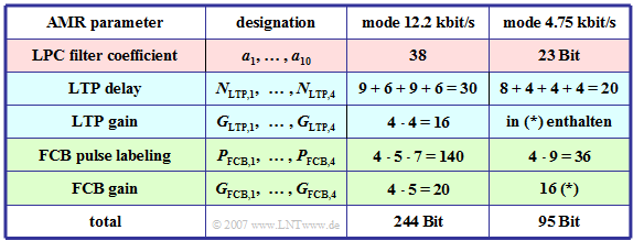
In the table, the parameters of the Adaptive Multi-Rate Codec are compiled for two modes:
- $244$ bits per $20 \ \rm ms$ ⇒ mode $12.2 \ \rm kbit/s$,
- $95$ Bit per $20 \ \rm ms$ ⇒ mode $4.75 \ \rm kbit/s$.
Algebraic Code Excited Linear Prediction
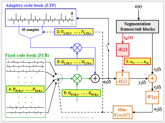
The graphic shows the ACELP based AMR codec. A short description of the principle follows. A detailed description can be found for example in [1].
- The voice signal $s(n)$, sampled at $8 \ \rm kHz$ and quantised at $13$ bit, as in the GSM fullrate speech codec, is divided into frames $s_{\rm R}(n)$ with $n = 1$, ..., before further processing. , $160$ or into subblocks $s_i(l)$ with $i = 1, 2, 3, 4$ and $l = 1$, ... , $40$ segmented.
- The calculation of the LPC coefficients is done in the red highlighted block frame by frame every $20 \ \rm ms$ corresponding to $160$ samples, since within this short time span the spectral envelope of the speech signal $s_{\rm R}(n)$ can be considered constant.
- For LPC analysis, a filter $A(z)$ of order $10$ is usually chosen. In the highest-rate mode with $12.2 \ \rm kbit/s$ the current coefficients $a_k \ ( k = 1$, ... , $10)$ of the short-time prediction are quantised every $10\ \rm ms$ , coded and made available for transmission at the point 1 highlighted in yellow.
- The further steps of the AMR are carried out every $5 \ \rm ms$ according to the $40$ samples of the signals $s_i(l)$ . The long-term prediction (LTP) - outlined in blue in the picture - is realised here as an adaptive codebook in which the samples of the preceding subblocks are entered.
- For the long-term prediction (LTP), first the gain $G_{\rm FCB}$ for the Fixed Code Book (FCB) is set to zero, so that a sequence of $40$ samples of the adaptive code book are present at the input $u_i(l)$ of the speech tract filter set by the LPC $A(z)^{-1}$ . The index $i$ denotes the subblock under consideration.
- By varying the two LTP parameters $N_{{\rm LTP},\hspace{0.05cm}i}$ and $G_{{\rm LTP},\hspace{0.05cm}i}$ shall be achieved for this $i$-th subblock that the root mean square - i.e. the mean power - of the weighted error signal $w_i(l)$ becomes minimal.
- The error signal $w_i(l)$ is equal to the difference between the current speech frame $s_i(l)$ and the output signal $y_i(l)$ of the so-called speech tract filter when excited with $u_i(l)$, taking into account the weighting filter $W(z)$ to match the spectral characteristics of human hearing.
- In other words, $W(z)$ removes those spectral components in the signal $e_i(l)$ that are not perceived by an "average" ear. In the mode $12.2 \ \rm kbit/s$ one uses $W(z) = A(z/γ_1)/A(z/γ_2)$ with constant factors $γ_1 = 0.9$ and $γ_2 = 0.6$.
- For each subblock, denotes $N_{{\rm LTP},\hspace{0.05cm}i}$ the best possible LTP delay, which together with the LTP gain $G_{{\rm LTP},\hspace{0.05cm}i}$ after averaging with respect to $l = 1$, ... , $40$ minimises the squared error $\text{E}[w_i(l)^2]$ . Dashed lines indicate control lines for iterative optimisation.
- The procedure described is called analysis by synthesis. After a sufficiently large number of iterations, the subblock $u_i(l)$ is included in the adaptive codebook. The determined LTP parameters $N_{{\rm LTP},\hspace{0.05cm}i}$ and $G_{{\rm LTP},\hspace{0.05cm}i}$ are encoded and made available for transmission.
Fixed Code Book – FCB
Nach der Ermittlung der besten adaptiven Anregung erfolgt die Suche nach dem besten Eintrag im festen Codebuch (Fixed Code Book, FCB).
- Dieses liefert die wichtigste Information über das Sprachsignal.
- Zum Beispiel werden beim $12.2 \ \rm kbit/s$–Modus hieraus pro Subblock $40$ Bit abgeleitet.
- Somit gehen in jedem Rahmen von $20$ Millisekunden $160/244 ≈ 65\%$ der Codierung auf den im Bild auf der letzten Seite grün umrandeten Block zurück.
Das Prinzip lässt sich anhand der Grafik in wenigen Stichpunkten wie folgt beschreiben:
- Im festen Codebuch kennzeichnet jeder Eintrag einen Puls, bei dem genau $10$ der $40$ Positionen mit $+1$ bzw. $-1$ belegt sind. Erreicht wird dies gemäß der Grafik durch fünf Spuren mit jeweils acht Positionen, von denen genau zwei die Werte $±1$ aufweisen und alle anderen Null sind.
- Ein roter Kreis in obiger Grafik $($an den Positionen $2,\ 11,\ 26,\ 30,\ 38)$ kennzeichnet eine $+1$ und ein blauer eine $-1$ $($im Beispiel bei $13,\ 17,\ 19,\ 24,\ 35)$. In jeder Spur werden die beiden belegten Positionen mit lediglich je drei Bit codiert (da es nur acht mögliche Positionen gibt).
- Für das Vorzeichen wird ein weiteres Bit verwendet, welches das Vorzeichen des erstgenannten Impulses definiert. Ist die Pulsposition des zweiten Impulses größer als die des ersten, so hat der zweite Impuls das gleiche Vorzeichen wie der erste, ansonsten das entgegengesetzte.
- In der ersten Spur des obigen Beispiels gibt es positive Pulse auf Position $2 \ (010)$ und Position $5 \ (101)$, wobei die Positionszählung bei $0$ beginnt. Diese Spur ist also gekennzeichnet durch die Positionen $010$ und $101$ sowie das Vorzeichen $1$ (positiv).
- Die Kennzeichnung für die zweite Spur lautet: Positionen $011$ und $000$, Vorzeichen $0$. Da hier die Pulse an Position $0$ und $3$ unterschiedliche Vorzeichen haben, steht $011$ vor $000$. Das Vorzeichen $0$ ⇒ negativ bezieht sich auf den Puls an der erstgenannten Position $3$.
- Ein jeder Puls – bestehend aus $40$ Impulsen, von denen allerdings $30$ das Gewicht "Null" besitzen – ergibt ein stochastisches, rauschähnliches Akustiksignal, das nach Verstärkung mit $G_{{\rm LTP},\hspace{0.05cm}i}$ und Formung durch das LPC–Sprachtraktfilter $A(z)^{–1}$ den Sprachrahmen $s_i(l)$ approximiert.
Aufgaben zum Kapitel
Aufgabe 3.5: GSM–Vollraten–Sprachcodec
Aufgabe 3.6: Adaptive Multi–Rate Codec
References
- ↑ 1.0 1.1 1.2 1.3 Kaindl, M.: Channel coding for voice and data in GSM systems. Dissertation. Chair of Communications Engineering, TU Munich. VDI Fortschritt-Berichte, Series 10, No. 764, 2005.
- ↑ Hindelang, T.: Source-Controlled Channel Decoding and Decoding for Mobile Communications. Dissertation. Chair of Communications Engineering, TU Munich. VDI Fortschritt-Berichte, Series 10, No. 695, 2002.
