Markov Chains

Considered scenario

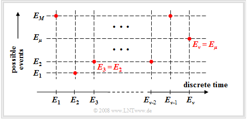
Finally, we consider the case where one runs a random experiment continuously and that at each discrete time $(ν = 1, 2, 3, \text{...})$ a new event $E_ν$. Here, let hold:

Possible events and event sequence

$$E_\nu \in G = \{ E_{\rm 1}, E_{\rm 2}, \hspace{0.1cm}\text{...}\hspace{0.1cm}, E_\mu , \hspace{0.1cm}\text{...}\hspace{0.1cm}, E_M \}.$$

This mathematically not quite proper nomenclature means (see graph):

The $M$ possible events are numbered consecutively with the index $μ$.
The index $ν$ names the discrete time points at which events occur.

For simplicity, we restrict ourselves in the following to the case $M = 2$ with the universal set $G = \{ A, \ B \}$. Let further hold:

The probability of event $E_ν$ may well depend on all previous events – that is, on the events $E_{ν\hspace{0.05cm}-1}, \hspace{0.15cm} E_{ν\hspace{0.05cm}-2}, \hspace{0.15cm} E_{ν\hspace{0.05cm}-3}$, and so on.
This statement also means that in this chapter we consider a sequence of events with internal statistical ties.

This scenario is a special case of a discrete-time, discrete-value random process, which will be discussed in more detail in the chapter Random Processes.

$\text{Example 1:}$ Cards are drawn one after the other from a deck of $32$ cards (including four aces). With the events

$A\text{ :}=$ "the drawn card is an ace", and
$B = \overline{A}:=$ "the drawn card is not an ace", the probabilities at time $ν = 1$:

$${\rm Pr} (A_{\rm 1}) ={4}/{32}= {1}/{8}, \hspace{0.5cm}{\rm Pr} (B_{\rm 1}) = {28}/{32}= {7}/{8}.$$

The probability ${\rm Pr} (A_{\rm 2})$, that an ace is drawn as the second card $(ν = 2)$ now depends on,

whether an ace was drawn at time $ν = 1$ ⇒ ${\rm Pr} (A_{\rm 2}) = 3/31 < 1/8$, or
whether at time $ν = 1$ no ace was drawn ⇒ ${\rm Pr} (A_{\rm 2}) = 4/31 > 1/8$.

Also, the probabilities ${\rm Pr} (A_{\nu})$ at later times $ν$ always depend on the occurrence or non-occurrence of all previous events $E_1, \hspace{0.1cm}\text{...}\hspace{0.1cm} ,E_{ν\hspace{0.05cm}–1}$ .

General definition of a Markov chain

In special cases, which however occur very frequently, the scenario described above can be described by a Markov chain.

$\text{Definition:}$ A $k$-th order Markov Chain serves as a model for time- and value-discrete processes, where the event probabilities at time $ν$

depend on the previous events $E_{ν\hspace{0.05cm}–1}, \hspace{0.15cm}\text{...}\hspace{0.15cm}, E_{ν\hspace{0.05cm}–k}$, and
can be expressed by $M^{k+1}$ conditional probabilities.

The diagram illustrates this issue using $k = 2$ as an example.

Second order Markov chain

For $M = 2$ there are $2^{k+1}$ such conditional probabilities:

$${\rm Pr} ( E_\nu \hspace {0.05cm}\vert \hspace {0.05cm}E_{\nu {\rm -1 } },\hspace {0.15cm}\text{...}\hspace {0.15cm}, E_{\nu { -k } }).$$

With $E_{\nu }\in \{ A, B \}, \hspace {0.15cm}\text{...}\hspace {0.15cm}, E_{\nu { -k } } \in \{ A, B \}$ these are:

${\rm Pr} ( A_\nu \hspace {0.05cm}\vert \hspace {0.05cm}A_{\nu {\rm -1 } }, A_{\nu { -2 } })$, ${\rm Pr} ( B_\nu \hspace {0.05cm}\vert \hspace {0.05cm}A_{\nu {\rm -1 } }, A_{\nu { -2 } })$,

${\rm Pr} ( A_\nu \hspace {0.05cm}\vert \hspace {0.05cm}A_{\nu {\rm -1 } },B_{\nu { -2 } })$, ${\rm Pr} ( B_\nu \hspace {0.05cm}\vert \hspace {0.05cm}A_{\nu {\rm -1 } }, B_{\nu { -2 } })$,

${\rm Pr} ( A_\nu \hspace {0.05cm}\vert \hspace {0.05cm}B_{\nu {\rm -1 } }, A_{\nu { -2 } })$, ${\rm Pr} ( B_\nu \hspace {0.05cm}\vert \hspace {0.05cm}B_{\nu {\rm -1 } }, A_{\nu { -2 } })$,

${\rm Pr} ( A_\nu \hspace {0.05cm}\vert \hspace {0.05cm}B_{\nu {\rm -1 } }, B_{\nu { -2 } })$, ${\rm Pr} ( B_\nu \hspace {0.05cm}\vert \hspace {0.05cm}B_{\nu {\rm -1 } }, B_{\nu { -2 } })$.

Synthetically generated texts (German and English)

$\text{Example 2:}$ Natural languages are often describable by Markov chains, although the order $k$ tends to infinity.

In this example, however, texts are only approximated by second-order Markov chains.

The graphic shows two synthetically generated texts:

The left text was synthetically generated starting from a German book template with bindings up to second order.
For the right text, an English book template was used.

One recognizes despite the restriction to $k = 2$ many (short) German and/or English words and also that German words are on the average longer than English.

There is no meaningful content, but the structure of the respective language is recognizable.

First order Markov chain

In the following, we always restrict ourselves to the special case $k =1$ .

$\text{Definition:}$

In a First Order Markov Chain only the statistical binding to the last event is considered, which in practice is usually the strongest.

A binary first order Markov chain ⇒ universal set $G = \{ A, \ B \}$ has the following event probabilities at time $\nu$:

$${\rm Pr}(A_\nu) = {\rm Pr}(A_\nu \hspace{0.05cm} \vert \hspace{0.05cm}A_{\nu - 1}) \cdot {\rm Pr}(A_{\nu - 1}) \hspace{0.1cm} + \hspace{0.1cm} {\rm Pr}(A_\nu \hspace{0.05cm} \vert \hspace{0.05cm}B_{\nu - 1}) \cdot {\rm Pr}(B_{\nu - 1}) ,$$

$${\rm Pr}(B_\nu) = {\rm Pr}(B_\nu \hspace{0.05cm} \vert \hspace{0.05cm}A_{\nu - 1}) \cdot {\rm Pr}(A_{\nu - 1}) \hspace{0.1cm} + \hspace{0.1cm} {\rm Pr}(B_\nu \hspace{0.05cm} \vert \hspace{0.05cm}B_{\nu - 1}) \cdot {\rm Pr}(B_{\nu - 1}) .$$

Regarding these equations, we note:

${\rm Pr}(A_\nu)$ is shorthand for the probability that at time $ν$ the event $E_ν = A = \overline{B}$ occurs, and it holds:

$${\rm Pr}(B_\nu) = 1 - {\rm Pr}(A_\nu).$$

At each time there are four transition probabilities ${\rm Pr}(E_ν\hspace{0.05cm} |\hspace{0.05cm} E_{ν–1})$, but only two of them are independent, because it holds:

$${\rm Pr}(B_\nu \hspace{0.05cm} | \hspace{0.05cm}A_{\nu - 1}) = 1 - {\rm Pr}(A_\nu \hspace{0.05cm} | \hspace{0.05cm}A_{\nu - 1}), \hspace{0.5cm}{\rm Pr}(A_\nu \hspace{0.05cm} | \hspace{0.05cm}B_{\nu - 1}) = 1 - {\rm Pr}(B_\nu \hspace{0.05cm} | \hspace{0.05cm}B_{\nu - 1}).$$

Generalizing this last statement: For a Markov chain with $M$ events, there are exactly $M · (M – 1)$ independent transition probabilities at each time $ν$.

$\text{Example 3:}$ With the given transition probabilities

$${\rm Pr}(A_ν\hspace{0.05cm}\vert\hspace{0.05cm} A_{ν–1}) = 0.2 \hspace{0.3cm}\text{and}\hspace{0.3cm} {\rm Pr}(B_ν\hspace{0.05cm} \vert\hspace{0.05cm} B_{ν–1}) = 0.4,$$

the other two transition probabilities are also uniquely specified

$${\rm Pr}(B_ν\hspace{0.05cm} \vert\hspace{0.05cm} A_{ν–1}) = 1- 0.2 = 0.8 \hspace{0.3cm}\text{and}\hspace{0.3cm} {\rm Pr}(A_ν\hspace{0.05cm} \vert\hspace{0.05cm} B_{ν–1}) = 1- 0.4 = 0.6.$$

Homogeneous Markov chains

Applicability of Markov chains to practical problems is usually only given with further restrictive conditions.

$\text{Definition:}$

If all transition probabilities are independent of the time $ν$, the Markov chain is homogeneous.

In the case $M = 2$ we use the following abbreviations for this:

$${\rm Pr}(A \hspace{0.05cm} \vert \hspace{0.05cm}A) = {\rm Pr}(A_\nu \hspace{0.05cm}\vert \hspace{0.05cm}A_{\nu - 1}) , \hspace{0.5cm} {\rm Pr}(A \hspace{0.05cm} \vert\hspace{0.05cm}B) = {\rm Pr}(A_\nu \hspace{0.05cm} \vert \hspace{0.05cm}B_{\nu - 1}) ,$$

$${\rm Pr}(B \hspace{0.05cm} \vert\hspace{0.05cm}A) = {\rm Pr}(B_\nu \hspace{0.05cm} \vert \hspace{0.05cm}A_{\nu - 1}) , \hspace{0.5cm} {\rm Pr}(B \hspace{0.05cm} \vert \hspace{0.05cm}B) = {\rm Pr}(B_\nu \hspace{0.05cm} \vert \hspace{0.05cm}B_{\nu - 1}) .$$

Thus, the event probabilities of a binary homogeneous Markov chain, which are absolute probabilities in contrast to the conditional transition probabilities, are :

First order homogeneous Markov chain

$${\rm Pr}(A_\nu) = {\rm Pr}(A \hspace{0.05cm} | \hspace{0.05cm}A) \cdot {\rm Pr}(A_{\nu - 1}) \hspace{0.1cm} + \hspace{0.1cm} {\rm Pr}(A \hspace{0.05cm} | \hspace{0.05cm}B) \cdot {\rm Pr}(B_{\nu - 1}) ,$$

$${\rm Pr}(B_\nu) = {\rm Pr}(B \hspace{0.05cm} | \hspace{0.05cm}A) \cdot {\rm Pr}(A_{\nu - 1}) \hspace{0.1cm} + \hspace{0.1cm} {\rm Pr}(B \hspace{0.05cm} | \hspace{0.05cm}B) \cdot {\rm Pr}(B_{\nu - 1}) .$$

We can also read from the Markov diagram:

The sum of the outgoing arrows of an event is always one

$${\rm Pr}(A \hspace{0.05cm} | \hspace{0.05cm}A) + {\rm Pr}(B \hspace{0.05cm} | \hspace{0.05cm}A) =1,$$

$${\rm Pr}(A \hspace{0.05cm} | \hspace{0.05cm}B) + {\rm Pr}(B \hspace{0.05cm} | \hspace{0.05cm}B) =1.$$

The sums of the incoming arrows this restriction does not apply:

$$ 0 \le {\rm Pr}(A \hspace{0.05cm} | \hspace{0.05cm}A) + {\rm Pr}(A \hspace{0.05cm} | \hspace{0.05cm}B)\le 2,$$

$$0 \le {\rm Pr}(B \hspace{0.05cm} | \hspace{0.05cm}A) + {\rm Pr}(B \hspace{0.05cm} | \hspace{0.05cm}B)\le 2.$$

You can calculate and display the "transient behavior" of the event probabilities of such a binary Markov chain with the interactive applet (German) Event Probabilities of a First Order Markov Chain .

Stationary probabilities

Important properties of random processes are stationarity und ergodicity. Although these terms are not defined until the fourth main chapter "Random Variables with Statistical Dependence" , we apply them here already in advance to Markov chains.

$\text{Definition:}$ If, in addition to the transition probabilities, all event probabilities of a Markov chain are independent of the time $ν$, then the Markov chain is called stationary. One then omits the index $ν$ and writes in the binary case:

$${\rm Pr}(A_\nu ) = {\rm Pr}(A ) \hspace{0.5 cm} {\rm bzw.} \hspace{0.5 cm} {\rm Pr}(B_\nu ) = {\rm Pr}(B).$$

These quantities are also called the ergodic probabilities of the Markov chain.

Stationary Markov chains have the special features mentioned below:

To calculate the ergodic probabilities of a binary Markov chain $(M =2)$ one can use the following equations:

$${\rm Pr}(A) = {\rm Pr}(A \hspace{0.05cm} | \hspace{0.05cm}A) \cdot {\rm Pr}(A) \hspace{0.1cm} + \hspace{0.1cm} {\rm Pr}(A \hspace{0.05cm} | \hspace{0.05cm}B) \cdot {\rm Pr}(B) ,$$

$${\rm Pr}(B) = {\rm Pr}(B \hspace{0.05cm} | \hspace{0.05cm}A) \cdot {\rm Pr}(A) \hspace{0.1cm} + \hspace{0.1cm} {\rm Pr}(B \hspace{0.05cm} | \hspace{0.05cm}B) \cdot {\rm Pr}(B) .$$

Since these equations depend linearly on each other, one may use only one of them. For example, as the second equation of determination one may use:

$${\rm Pr}(A) + {\rm Pr}(B) = 1.$$

The ergodic probabilities result from it to

$${\rm Pr}(A) = \frac {{\rm Pr}(A \hspace{0.05cm} | \hspace{0.05cm}B) }{{\rm Pr}(A \hspace{0.05cm} | \hspace{0.05cm}B) + {\rm Pr}(B \hspace{0.05cm} | \hspace{0.05cm}A) }\hspace{0.1cm}, \hspace{0.5cm}{\rm Pr}(B) = \frac {{\rm Pr}(B \hspace{0.05cm} | \hspace{0.05cm}A) }{{\rm Pr}(A \hspace{0.05cm} | \hspace{0.05cm}B) + {\rm Pr}(B \hspace{0.05cm} | \hspace{0.05cm}A) }.$$

$\text{Example 4:}$ We consider a binary Markov chain with events $A$ and $B$ and transition probabilities ${\rm Pr}(A \hspace{0.05cm} \vert\hspace{0.05cm}A) = 0.4$ and ${\rm Pr}(B \hspace{0.05cm} \vert \hspace{0.05cm}B) = 0.8$.
Furthermore, we assume that each realization of this chain starts with event $A$ at the starting time $ν = 0$ .

We then obtain the event probabilities listed below (with three decimal places):

Zum Einschwingen der Ereigniswahrscheinlichkeiten

In a strict sense, this is a non-stationary Markov chain, but it is (nearly) settled after a short time:

At later times $(ν > 5)$ , the event probabilities ${\rm Pr}(A_ν) \approx 1/4$ and ${\rm Pr}(B_ν) \approx 3/4$ are no longer seriously changed.
However, from ${\rm Pr}(A_{ν=5}) = 0.250$ and ${\rm Pr}(B_{ν=5}) = 0.750$ it should not be concluded that the Markov chain is already perfectly steady at time $ν = 5$ .
Indeed, the exact values are ${\rm Pr}(A_{ν=5}) = 0.25024$ and ${\rm Pr}(B_{ν=5}) = 0.74976$.

$\text{Conclusion:}$ For a stationary Markov chain, the ergodic probabilities always occur with good approximation very long after the chain is switched on $(ν → ∞)$ , regardless of the initial conditions ${\rm Pr}(A_0)$ and ${\rm Pr}(B_0) = 1 - {\rm Pr}(A_0)$.

Matrix vector representation

Homogeneous Markov chains can be represented very compactly with vectors and matrices. This is especially recommended for more than two events:

$$E_\nu \in G = \{ E_{\rm 1}, E_{\rm 2}, \hspace{0.1cm}\text{...}\hspace{0.1cm}, E_\mu , \hspace{0.1cm}\text{...}\hspace{0.1cm}, E_M \}.$$

For the matrix-vector representation, we use the following nomenclature:

We summarize the $M$ probabilities at time $ν$ in a column vector:

$${\mathbf{p}^{(\nu)}} = \left[ \begin{array}{c} {p_{\rm 1}}^{(\nu)} \\ \dots \\ {p_{M}}^{(\nu)} \end{array} \right] \hspace{0.5cm}{\rm mit} \hspace{0.5cm} {p_{\mu}}^{(\nu)} = {\rm Pr}(E_\nu = E_\mu ).$$

The transition probabilities are expressed by an $M \times M$ matrix:

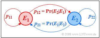
$${\mathbf{P}} =\left( p_{ij} \right) = \left[ \begin{array}{cccc} p_{11} & p_{12} & \cdots & p_{1M} \\ p_{21} & p_{22}& \cdots & p_{2M} \\ \dots & \dots & \dots & \dots \\ p_{M1} & p_{M2} & \cdots & p_{MM} \end{array} \right] \hspace{0.5cm}{\rm mit} \hspace{0.5cm} {p_{ij}} = {\rm Pr}(E_{\nu +1 } = E_j \hspace{0.05cm}| \hspace{0.05cm} E_{\nu } = E_i).$$

The accompanying figure illustrates this nomenclature using the example $M = 2$. The new event probability vector after one step is:

To denote the transition probabilities

$${\mathbf{p}^{(\nu + 1)}} = {\mathbf{P}}^{\rm T} \cdot {\mathbf{p}^{(\nu )}} .$$

Here,${\mathbf{P}^{\rm T}}$ denotes the transposed matrix to $\mathbf{P}$. Thus, after $n$ steps, the result is

$${\mathbf{p}^{(\nu +{\it n})}} = \left( {\mathbf{P}}^{\rm T} \right)^n \cdot {\mathbf{p}^{(\nu )}} .$$

In the limit transition $(n → ∞)$ one then always achieves stationarity of the Markov chain:

$$\lim_{n \to\infty}\hspace{0.1cm}{\mathbf{p}^{(\nu + n)}} = \lim_{n \to\infty} \left( {\mathbf{P}}^{\rm T} \right)^n \cdot {\mathbf{p}^{(\nu )}} = {\mathbf{p}}_{\rm erg}= \left[ \begin{array}{c} {p_{\rm 1}} \\ \dots \\ {p_{M}} \end{array} \right] .$$

$\text{Definition:}$ Multiplying the transition matrix ${\mathbf{P} }$ infinitely many times by itself and denoting the result by ${\mathbf{P} }_{\rm erg}$, the resulting matrix consists of $M$ equal rows:

$${\mathbf{P} }_{\rm erg} = \lim_{n \to\infty} {\mathbf{P} }^n = \left[ \begin{array}{cccc} p_{1} & p_{2} & \cdots & p_{M} \\ p_{1} & p_{2}& \cdots & p_{M} \\ \dots & \dots & \dots & \dots \\ p_{1} & p_{2} & \cdots & p_{M} \end{array} \right] .$$

The probabilities $p_1, \hspace{0.1cm}\text{...}\hspace{0.1cm}, p_M$ in each of these lines are called the ergodic probabilities.

Markov diagram with three events

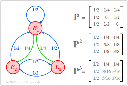
$\text{Example 5:}$ We consider a Markov chain with the events $E_1, E_2$ and $E_3$ ⇒ $M=3$. The graph shows

on the left the Markov diagram,
on the upper right the transition matrix $\mathbf{P}$ and
below their powers $\mathbf{P}^2$ and $\mathbf{P}^3$.

In the Markov diagram, all transition probabilities with the numerical value $1/2$ are shown in blue; green indicates the probability $1/4$.

At the start $(ν =0)$ all events are equally probable. For $ν = 1$ then holds:

$${\mathbf{p}^{(1)} } = {\mathbf{P} }^{\rm T} \cdot {\mathbf{p}^{(0 )} }= \left[ \begin{array}{ccc} 1/2 & 1/2& 1/2 \\ 1/4 & 0 & 1/2 \\ 1/4& 1/2& 0 \end{array} \right] \left[ \begin{array}{c} 1/3 \\ 1/3 \\ 1/3 \end{array} \right] = \left[ \begin{array}{c} 1/2 \\ 1/4 \\ 1/4 \end{array} \right] .$$

From this it can be seen that we get from the matrix $\mathbf{P}$ to the transposed matrix ${\mathbf{P}^{\rm T} }$ by exchanging the rows and columns.

At time $ν =2$ (and also at all later times) the same probabilities result:

$${\mathbf{p}^{(2)} } = {\mathbf{P} }^{\rm T} \cdot {\mathbf{p}^{(1 )} }= \left[ \begin{array}{ccc} 1/2 & 1/2& 1/2 \\ 1/4 & 0 & 1/2 \\ 1/4& 1/2& 0 \end{array} \right] \left[ \begin{array}{c} 1/2 \\ 1/4 \\ 1/4 \end{array} \right] = \left[ \begin{array}{c} 1/2 \\ 1/4 \\ 1/4 \end{array} \right] .$$

This means: the ergodic probabilities of the three events are $1/2$ $($for $E_1)$, $1/4$ $($for $E_2)$, and $1/4$ $($for $E_3)$.

This result could have been read directly from the ergodic matrix:

$${\mathbf{P} }_{\rm erg} = \lim_{n \to\infty} {\mathbf{P} }^n = \left[ \begin{array}{ccc} 1/2 & 1/4 & 1/4 \\ 1/2 & 1/4 & 1/4 \\ 1/2 & 1/4 & 1/4 \end{array} \right] .$$

This is obtained by continuously multiplying the transition matrix by itself.