Viterbi Receiver

1 Considered scenario and prerequisites
2 Error quantities and total error quantities
3 Minimum total error quantities
4 Representation of the minimum total error quantities – Trellis diagram
5 Simplified trellis diagram
6 Extension to two precursors
7 Error probability in maximum likelihood decision
8 Exercises for the chapter

Considered scenario and prerequisites

The "correlation receiver" is optimal in the sense of the "maximum likelihood decision rule", that is, it leads to the minimum error probability for equally likely source symbols. Disadvantage:

Block diagram of the Viterbi receiver

The realization cost increases exponentially with the length $N$ of the symbol sequence to be detected.

Since the sequence is decided jointly, long delays occur when $N$ is large.

In the 1970s, Andrew J. Viterbi proposed a maximum likelihood receiver that allows detection of parts of the received message and for which the implementation cost is limited even for infinitely long sequences.

It should be noted with regard to the individual components of the block diagram:

Adjusted to the basic reception pulse $g_r(t)$ and the noise, the "matched filter" $H_{\rm MF}(f)$ serves for "noise power limitation". The matched filter output signal $m(t)$ or the sequence $\langle m_\nu \rangle$ of equidistant signal values after sampling has the best possible signal-to-noise power ratio $\rm (SNR)$.

The task of the decorrelation filter $H_{\rm DF}(f)$ is to extract from the sequence $\langle m_\nu \rangle$ the detection samples $d_\nu = d_{{\rm S}\nu} + d_{{\rm N}\nu}$ whose noise components $d_{{\rm N}\nu}$ are uncorrelated. This filter is therefore also called a "whitening filter".

The Viterbi decision, which is the focus of the following considerations, obtains the binary output sequence $\langle v_\nu \rangle$ from the continuous-valued input sequence $\langle d_\nu \rangle$ according to the maximum likelihood rule with the smallest possible error probability ${\rm Pr}(v_\nu \ne q_\nu)$.

In order to describe the Viterbi algorithm as simply as possible, some simplifying assumptions are made here:

Let the amplitude coefficients be unipolar ⇒ $a_\nu \in \{0,\hspace{0.05cm} 1\}$. Note that using bipolar coefficients ⇒ $a_\nu \in \{-1,\hspace{0.05cm} +1\}$ requires only a few modifications. These difficulties concern the description rather than the implementation.
The basic pulse $g_d(t)$ after the decorrelation filter $H_{\rm DF}(f)$ consists only of the main value $g_0 = g_d(t = T_{\rm D})$ and a single precursor $g_{-1} = g_d(t = T_{\rm D}-T)$. There are no trailers ("postcursors") in our model: $g_{\nu} = g_d(t = T_{\rm D}+\nu \cdot T)\equiv0$. Also, let other precursors be excluded for now: $g_{-2} = g_{-3}= \text{ ...} = 0$.
This gives for the samples of the continuous decorrelation filter output signal $d(t)$ at time $\nu \cdot T$: $d_{\nu} = a_{\nu}\cdot g_{0} + a_{\nu+1}\cdot g_{-1}+d_{{\rm N}\nu}\hspace{0.05cm}$, where the noise component $d_{{\rm N}\nu}$ is assumed to be Gaussian distributed with standard deviation $\sigma_d$.

Note: The algorithm is not more complex with bipolar signaling. $\bullet$ In contrast, the computational cost increases when the basic detection pulse becomes broader and has more than one precursor $g_{-1}$. $\bullet$ The neglect of precursors in the description is not a fundamental limitation because any pulse can satisfy this condition by appropriate choice of the detection time $T_{\rm D}$. $\bullet$ In the following all signal values are normalized to $1$.

$\text{Example 1:}$ In the graph, the samples $d_{ {\rm S}\nu}$ of the noiseless detection signal are entered as (blue) crosses, where the corresponding amplitude coefficients $a_1 = 1$, $a_2 = 1$, $a_3 = 0$, ... can be read from the source signal $q(t)$ plotted in green.

Sampling values to illustrate the Viterbi algorithm

The basic pulse values are assumed to be $g_0 = 0.7$ and $g_{-1} = 0.3$. It can be further seen that $d_{ {\rm S}\nu}$ can take only four different values, namely $0$, $g_{-1}=0.3$, $g_0= 0.7$, $g_0 +g_{-1}= 1$.

The noisy samples present at the Viterbi decision (red dots) are $d_0 = 0.2$, $d_1 = 0.7$, $d_2 = 0.5$, $d_3 = 0$, ... , where the differences $d_{ {\rm N}\nu} = d_\nu - d_{ {\rm S}\nu}$ originate from an AWGN noise source.

A threshold decision $($with the threshold at $E = 0.5)$ would make at least one wrong decision at these ten bits shown $($at time $t = 4T)$, and possibly another at $t = 2T$ if the sample $d_2 = 0.5$ is nevertheless slightly smaller than the threshold $E = 0.5$.
In contrast, the Viterbi receiver will correctly decide this sequence of length $10$, as shown in the next sections.

Error quantities and total error quantities

As in the chapter "Optimal Receiver Strategies", $Q \in \{Q_i\}$ specifies the time-limited source symbol sequence consisting of $N$ binary symbols.

Thus, the number of possible symbol sequences $Q_i$ is $2^N$.

$V$ denotes the sink symbol sequence of length $N$ set equal to the most probable sequence $Q_j$ by the Viterbi decision.

$\text{Definitions:}$

The error quantity $\varepsilon_{\nu}(i)$ denotes the squared deviation between the actual noisy sample $d_\nu$ and the noiseless sample $d_{ {\rm S}\nu}$ belonging to the sequence $Q_i$:

$$\varepsilon_{\nu}(i) = \vert d_{\nu} - d_{ {\rm S}\nu}(i) \vert^2 \hspace{0.05cm}.$$

In the literature, this is also referred to as "metric".

The total error quantity $\gamma_{\nu}(i)$ characterizes the sum of all error quantities up to time $\nu$:

$$\gamma_{\nu}(i)= \sum_{k=0}^{\nu}\varepsilon_{k}(i) \hspace{0.05cm}.$$

In this context, one also speaks of the "accumulated metric".

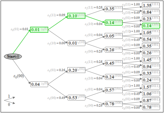
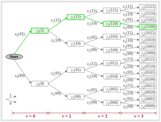
The graph illustrates the quantities defined above in a tree structure, from which it can be seen that the total error quantities can be calculated iteratively:

Representation of the error quantities $\varepsilon_{\nu}(i)$ and accumulated error quantities $\gamma_{\nu}(i)= \gamma_{\nu-1}(i\hspace{0.05cm}')+\varepsilon_{\nu}(i\hspace{0.05cm}'') \hspace{0.05cm}$ in the tree diagram. Notes:
$\bullet$ $i$, $i\hspace{0.05cm}'$, $i\hspace{0.05cm}''$ are different index variables.
$\bullet$ Definition is valid for a basic pulse with main value $g_{0}$ and precursor $g_{-1}$.
$\bullet$ With $v$ precursors the above sum would have to start at $k = 1 -v$.
$\bullet$ The parameter $i \in \{0, \hspace{0.05cm}\text{...} \hspace{0.05cm}, 2^{N+1}-1\}$ is usually represented in binary.
$\bullet$ It describes the amplitude coefficients $a_1$, ... , $a_{\nu +1}$ $($each $0$ or $1)$.

$$\gamma_{\nu}(i)= \gamma_{\nu-1}(i\hspace{0.05cm}')+\varepsilon_{\nu}(i\hspace{0.05cm}'') \hspace{0.05cm}.$$

It should be noted about this graph:

The nodes of the tree diagram represent the "total error quantities" $\gamma_{\nu}(i)$. Their number is doubled with each iteration step. At time $\nu$, there are $2^{\nu+1}$ such nodes. For example, for $\nu = 3$, exactly $2^4 = 16$ nodes can be seen.

The "amplitude coefficients" associated with the total error quantities $\gamma_{\nu}(i)$ are obtained by following the path from the initial node to the node under consideration. It is agreed that an upward branch is assigned the coefficient $a_\nu=1$ and a downward branch is assigned the coefficient $a_\nu=0$.

The green highlighted node $\gamma_{3}(\rm 1100)$ denotes the total error quantity under the hypothetical assumption that the symbols $a_1=1$, $a_2=1$, $a_3=0$, $a_4=0$ were sent. This assignment can also be read from the directions of the arrows in the tree diagram: First twice upwards, then twice downwards.

Due to the precursor, the coefficient $a_4$ must already be taken into account at time $\nu = 3$. All nodes $\gamma_{\nu}(i)$ computed under the assumption $a_{\nu +1}=1$ are represented by rectangles, while the hypothesis $a_{\nu +1}=0$ is symbolized by a rounded rectangle in each case, for example $\gamma_{2}(\rm 110)$ or $\gamma_{3}(\rm 1100)$.

The branches in the tree diagram are assigned to "error quantities" $\varepsilon_{\nu}(i)$. With the assumed basic pulse $($only $g_{0}$ and $g_{-1})$, there are exactly four different quantities at each time point except for the initial state $(\nu = 0)$:

$$\varepsilon_{\nu}(00) = |d_{\nu}|^2\hspace{0.05cm},\hspace{0.5cm}\varepsilon_{\nu}(01) = |d_{\nu}-g_{-1}|^2\hspace{0.05cm},$$

$$ \varepsilon_{\nu}(10) = |d_{\nu}-g_{0}|^2\hspace{0.05cm},\hspace{0.2cm}\varepsilon_{\nu}(11) = |d_{\nu}-g_{0}-g_{-1}|^2\hspace{0.05cm}.$$

The total error quantity $\gamma_{\nu}(i)$ is the sum of the preceding node $\gamma_{\nu-1}(i\hspace{0.05cm}')$ and the intervening branch $\varepsilon_{\nu}(i\hspace{0.05cm}'')$. For example, for the highlighted nodes:

$$\gamma_{1}(11)=\gamma_{0}(1)+\varepsilon_{1}(11) ,$$

$$ \gamma_{2}(110)=\gamma_{1}(11)+\varepsilon_{2}(10) ,$$

$$ \gamma_{3}(1100)=\gamma_{2}(110)+\varepsilon_{3}(00).$$

For the first nodes $\gamma_{0}(0)$ and $\gamma_{0}(1)$, it is considered that, by convention, the symbol $a_0=0$ is always transmitted before the actual transmission $(a_1$, $a_2$, ...$)$. It follows that:

$$\gamma_{0}(0)=\varepsilon_{0}(00)= |d_{0}|^2 \hspace{0.05cm},\hspace{0.2cm} \gamma_{0}(1)=\varepsilon_{0}(01)=|d_{0}-g_{-1}|^2 \hspace{0.05cm}.$$

The following two examples will hopefully clarify these somewhat tedious statements.

$\text{Example 2:}$ As in $\text{Example 1}$, we consider the unipolar source symbol sequence of length $N=3$ with the following parameter values:

$$g_{0}=0.7 \hspace{0.05cm},\hspace{0.2cm} g_{-1}=0.3 \hspace{0.05cm},\hspace{0.2cm} d_{0}=0.2 \hspace{0.05cm},\hspace{0.2cm} d_{1}=0.7 \hspace{0.05cm},\hspace{0.2cm} d_{2}=0.5 \hspace{0.05cm},\hspace{0.2cm} d_{3}=0 \hspace{0.05cm} \hspace{0.05cm}.$$

Then, for the error quantities $\varepsilon_{\nu}(i)$ at time points $\nu = 0$ to $\nu = 3$:

$$\nu = 0\text{:} \hspace{0.2cm}\varepsilon_{0}(00) = \big [0.2- (0 \cdot 0.7 + 0 \cdot 0.3) \big ]^2=0.04 \hspace{0.05cm},\hspace{0.4cm} \varepsilon_{0}(01) = \big [0.2- (0 \cdot 0.7 + 1 \cdot 0.3) \big ]^2=0.01 \hspace{0.05cm};$$

$$\nu = 1{:} \hspace{0.2cm}\varepsilon_{1}(00) = \big [0.7- (0 \cdot 0.7 + 0 \cdot 0.3)\big ]^2=0.49 \hspace{0.05cm},\hspace{0.4cm} \varepsilon_{1}(01) = \big [0.7- (0 \cdot 0.7 + 1 \cdot 0.3)\big ]^2=0.16 \hspace{0.05cm},$$

$$\hspace{1.4cm}\varepsilon_{1}(10) = \big [0.7- (1 \cdot 0.7 + 0 \cdot 0.3)\big ]^2=0.00 \hspace{0.05cm}\hspace{0.4cm}\varepsilon_{1}(11) = \big [0.7- (1 \cdot 0.7 + 1 \cdot 0.3)\big ]^2=0.09 \hspace{0.05cm};$$

$$\nu = 2\text{:} \hspace{0.2cm}\varepsilon_{2}(00) = \big [0.5- (0 \cdot 0.7 + 0 \cdot 0.3)\big ]^2=0.25 \hspace{0.05cm},\hspace{0.4cm}\varepsilon_{2}(01) = \big [0.5- (0 \cdot 0.7 + 1 \cdot 0.3)\big ]^2=0.04 \hspace{0.05cm},$$

$$\hspace{1.4cm}\varepsilon_{2}(10) = \big [0.5- (1 \cdot 0.7 + 0 \cdot 0.3)\big ]^2=0.04 \hspace{0.05cm},\hspace{0.4cm}\varepsilon_{2}(11) = \big [0.5- (1 \cdot 0.7 + 1 \cdot 0.3)\big ]^2=0.25 \hspace{0.05cm};$$

$$ \nu = 3\text{:} \hspace{0.2cm}\varepsilon_{3}(00) = \big [0.0- (0 \cdot 0.7 + 0 \cdot 0.3)\big ]^2=0.00 \hspace{0.05cm},\hspace{0.4cm}\varepsilon_{3}(01) = \big [0.0- (0 \cdot 0.7 + 1 \cdot 0.3)\big ]^2=0.09 \hspace{0.05cm},$$

$$\hspace{1.4cm}\varepsilon_{3}(10) = \big [0.0- (1 \cdot 0.7 + 0 \cdot 0.3)\big ]^2=0.49 \hspace{0.05cm},\hspace{0.4cm}\varepsilon_{3}(11) = \big [0.0- (1 \cdot 0.7 + 1 \cdot 0.3)\big ]^2=1.00 \hspace{0.05cm}.$$

$\text{Example 3:}$ With the error quantities $\varepsilon_{\nu}(i)$ determined in $\text{Example 2}$, the total error quantities $\gamma_{\nu}(i)$ can now also be calculated. Below is the tree diagram with the total error quantities $\gamma_{\nu}(i)$ as nodes for the time points $\nu = 0$ to $\nu = 3$.

Iterative calculation of the total error quantities (example)

The minimum total error quantity at time $\nu = 3$ is $\gamma_{3}(\rm 1100) = 0.14$. From this, the coefficients of the most likely transmitted (unipolar) sequence according to the present signal values $d_0 = 0.2$, $d_1 = 0.7$, $d_2 = 0.5$ and $d_3 = 0$ are $a_1 = 1$, $a_2 = 1$ and $a_3 = 0$ (green path).

Further, it should be noted:

If the sequence length is $N = 3$ (that is: only three symbols are jointly decided by the Viterbi receiver), the decision $a_4 = 0$ is also certainly the correct one, since all coefficients $a_{\nu>3}$ were assumed to be zero.

However, for longer sequences $(N > 3)$, it cannot necessarily be concluded from the minimum value $\gamma_{3}(\rm 1100)$ that $a_1 = 1$, $a_2 = 1$, $a_3 = 0$ is actually part of the most probable sequence. Considering further sample values $(d_4$, $d_5$, ...$)$ this preliminary result could well change.

Minimum total error quantities

Simplification of the tree diagram according to Viterbi

We continue from the numerical values of the last examples:

$$d_{0}=0.2 ,\hspace{0.1cm} d_{1}=0.7 ,\hspace{0.1cm} d_{2}=0.5 ,\hspace{0.1cm} d_{3}=0 ,$$

$$g_{0}=0.7 ,\hspace{0.1cm} g_{-1}=0.3 .$$

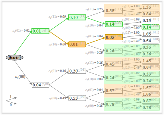
Thus, nothing changes in the tree diagram compared to $\text{Example 3}$. Some colored markings in this diagram only indicate in which way the tree diagram can be simplified according to Viterbi's suggestions.

Important properties of the Viterbi decision can be seen in the above graph, for example, at time $\nu = 2$:

At time $\nu = 2$, the minimum total error quantity is $\gamma_{2}(\rm 101) = 0.05$ (highlighted in brown). This means: A decision at $\nu = 2$ – based on $d_0$, $d_1$ and $d_2$ – would have been in favor of sequence $\rm 101$ instead of the transmitted sequence $\rm 110$.

It follows: A too early final determination should be avoided at all costs. However, at any time $\nu$ one can already exclude several partial symbol sequences which need not be considered at later times.

To $\gamma_{2}(\rm 111) = 0.35$ the same error quantities $\varepsilon_{3}(\rm 11)$ and $\varepsilon_{3}(\rm 10)$ are added as to $\gamma_{2}(\rm 101) = 0.05$. Because of $\gamma_{2}(\rm 111) > \gamma_{2}(\rm 101)$ it is therefore already certain at $\nu = 2$ that $\rm 111$ cannot be part of the most probable sequence. The same is true for $\rm 001$ and $\rm 011$. Therefore, these nodes and all their successors need not be considered further (brown overlaps).

Also, the rounded nodes $\gamma_{2}(\rm 000) = 0.78$, $\gamma_{2}(\rm 010) = 0.24$ and $\gamma_{2}(\rm 100) = 0.26$ are not part of the most probable sequence, since they are larger than the node $\gamma_{2}(\rm 110) = 0.14$, which is marked in green. Also, these and their successors need not be considered from time $\nu = 3$ (green covers).

$\text{Conclusion:}$

Of the eight nodes at $\nu = 2$, only two need to be followed up, namely the rectangle $\gamma_{2}(\rm 101) = 0.05$ and the rounded rectangle $\gamma_{2}(\rm 110) = 0.14$.
These describe the minimum total error quantities assuming that $a_3 = 0$ and $a_3 = 1$, respectively.

Representation of the minimum total error quantities – Trellis diagram

We now generalize the result of this example. Under the still valid assumption that the basic pulse has only one precursor $(g_{-1})$ besides the main value $(g_0)$, the two minimum total error quantities at time $\nu$ are formally given by

$${\it \Gamma}_{\nu}(0) = {\rm Min}\left[{\it \Gamma}_{\nu-1}(0) + \varepsilon_{\nu}(00), \hspace{0.2cm}{\it \Gamma}_{\nu-1}(1) + \varepsilon_{\nu}(10)\right] \hspace{0.05cm},$$

$${\it \Gamma}_{\nu}(1) = {\rm Min}\left[{\it \Gamma}_{\nu-1}(0) + \varepsilon_{\nu}(01), \hspace{0.2cm}{\it \Gamma}_{\nu-1}(1) + \varepsilon_{\nu}(11)\right] \hspace{0.05cm}.$$

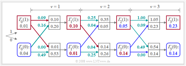
The total error minimization procedure can be clearly illustrated in the trellis diagram.

Example trellis diagram

A comparison with the figures in the last sections shows:

The lower branch represents the minimum total error quantity ${\it \Gamma}_{\nu}(0)$ calculated at each time $\nu$ under the hypothesis that $a_{\nu + 1} = 0$ will hold (blue rounded squares).

In contrast, the upper branch describes the minimum total error quantities ${\it \Gamma}_{\nu}(1)$ under the assumption $a_{\nu + 1} = 1$ (red squares). Again, the numerical values are adapted to the previous example.

Besides ${\it \Gamma}_{\nu}(0)$ and ${\it \Gamma}_{\nu}(1)$, the maximum likelihood decision must also store the associated symbol sequences (paths). These branches are highlighted in red and blue, respectively, in the graph.

If ${\it \Gamma}_{\nu}$ arises from the node ${\it \Gamma}_{\nu-1}(0)$ – that is, if the lower of the two incoming branches is highlighted – the associated symbol is $\rm 0$, otherwise the symbol is $\rm 1$.

At time $\nu = 3$, for example, both ${\it \Gamma}_{3}(0) = 0.14$ and ${\it \Gamma}_{3}(1) = 0.23$ result from the precursor ${\it \Gamma}_{2}(0)$, so that both selected paths point to the symbol $\rm 0$, respectively (blue branches).

Simplified trellis diagram

The advantage of the trellis diagram is that the number of nodes and branches does not double at each iteration step. By selecting the minimum total error quantities, only those symbol sequences are considered further which can be considered as part of the most probable sequence at all.

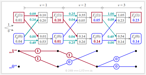
The trellis diagram can be further simplified by drawing in only the selected branches. This is illustrated in the lower part of the diagram with our numerical example. As a reminder: The actual transmitted amplitude coefficients are $a_1= 1$, $a_2= 1$ and $a_3= 0$, and the trellis diagram drawn above was calculated assuming that due to the pulse values $g_{-1} = 0.3$ and $g_{0} = 0.7$ as well as the AWGN noise, the input values $d_0= 0.2$, $d_1= 0.7$, $d_2= 0.5$ and $d_3= 0$ are applied to the ML decision.

Trellis diagram and simplified trellis diagram

This simplified trellis diagram allows the following statements:

The decision about $a_1= 1$ can be made immediately at the time $\nu = 1$, since under both hypotheses – namely the following symbol is $a_2= 0$ or this symbol is $a_2= 1$ – the same result $a_1= 1$ is obtained.

In contrast, at the time $\nu = 2$ the final decision about $a_2$ cannot yet be made. Assuming that $a_3= 0$, one would have to decide for $a_2= 1$, while the hypothesis $a_3= 1$ would lead to the fixed choice of $a_2= 0$.

At time $\nu = 3$ the decision for $a_1= 1$, $a_2= 1$, $a_3= 0$ is final, since both continuous paths suggest this (the correct in this case) sequence.
If one were to postpone the decision to time $\nu = 4$, one would no longer have usable information about $a_1$, $a_2$ and $a_3$ available.

All statements in this chapter can be verified with the interactive applet "Viterbi receiver for one precursor".

Extension to two precursors

If the basic pulse is described by the samples $g_{0} \ne 0$, $g_{-1} \ne 0$ and $g_{-2} \ne 0$, then four metrics ${\it \Gamma}_{\nu}(00)$, ${\it \Gamma}_{\nu}(01)$, ${\it \Gamma}_{\nu}(10)$ and ${\it \Gamma}_{\nu}(11)$ must be determined in the trellis diagram at each time $\nu$. For example, ${\it \Gamma}_{\nu}(01)$ then describes the minimum total error quantity for the detection of the symbol $a_\nu$ under the hypothesis that $a_{\nu-1} = 0$ and $a_{\nu-2} = 1$, and it holds:

$${\it \Gamma}_{\nu}(01) = {\rm Min}\big[{\it \Gamma}_{\nu-1}(00) + \varepsilon_{\nu}(001), \hspace{0.2cm}{\it \Gamma}_{\nu-1}(10) + \varepsilon_{\nu}(101)\big] \hspace{0.05cm}.$$

Exercise 3.12 discusses in detail the calculation of error quantities (metrics) and the minimization of total error quantities (accumulated metrics).

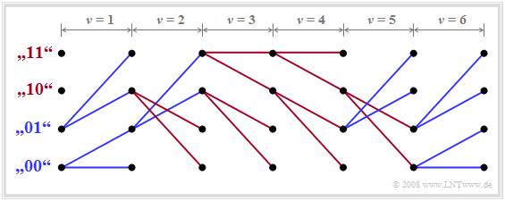
$\text{Example 4:}$ We consider here an exemplary trellis diagram, which reflects the (error-free) detection of the following symbol sequence:

$$a_{1}=0 \hspace{0.05cm},\hspace{0.2cm} a_{2}=0 \hspace{0.05cm},\hspace{0.2cm} a_{3}=1 \hspace{0.05cm},\hspace{0.2cm} a_{4}=1 \hspace{0.05cm},\hspace{0.2cm} a_{5}=1 \hspace{0.05cm},\hspace{0.2cm} a_{6}=0 \hspace{0.05cm}, \hspace{0.05cm}\text{...}$$

Trellis diagram for two precursors

This simplified trellis diagram allows the following statements:

All branches departing from ${\it \Gamma}_{\nu}(00)$ or ${\it \Gamma}_{\nu}(01)$ are assigned to symbol $\rm 0$ and drawn in blue. The red branches departing from the two upper states denote symbol $\rm 1$.

If one follows the continuous paths, one recognizes the indicated sequence. Since at the time $\nu = 6$ only blue branches arrive, the first six bits of the sequence are finally fixed here.

However, partial sequences could also be output already at times $\nu = 1$, $\nu = 3$ and $\nu = 4$, since at these times the same partial paths result for all four states.

In contrast, at $\nu = 2$ and $\nu = 5$, decisions may not be made immediately. For example, at time $\nu = 5$ it is only certain that either $a_5 = 0$ and $a_6 = 1$ will be or $a_5 = 1$ and $a_6 = 0$. Other combinations are not possible.

Error probability in maximum likelihood decision

The exact error probability calculation in ML decision (for example with the correlation or the Viterbi receiver) is very complex. Thereby

determine the difference energies between all possible symbol sequences $Q_i$ and $Q_{j \ne i}$, where the error probability is essentially determined by the minimum difference energy;

also the influences of matched filter $H_{\rm MF}(f)$ and decorrelation filter $H_{\rm DF}(f)$ are taken into account and additionally the rms value $\sigma_d$ of the detection noise signal is determined.

$\text{Without proof:}$ A simple approximation for the (average) error probability in maximum likelihood decision is:

$$p_{\rm ML} = {\rm Q}\left(g_{\rm max}/{\sigma_d}\right) \hspace{0.3cm}{\rm with}\hspace{0.2cm}g_{\rm max}= {\rm Max}\hspace{0.15cm} \vert g_\nu \vert \hspace{0.05cm}.$$

The approximation is valid only for binary bipolar signaling. For unipolar signaling, the argument of the Q function must be halved.

For the following interpretation and example, it is assumed that $v + 1$ basic pulse values (including the main value) are different from zero. Then holds:

The Viterbi decision must consider all these basic pulse values. This means that a trellis diagram with $2^v$ states has to be processed.

The precondition for the validity of the above equation is the uncorrelatedness of the noise at the decision, which is achieved by the decorrelation filter.

For the comparison with threshold decision $(p_{\rm SE})$ or decision feedback $(p_{\rm DFE})$ the noise rms value $\sigma_d$ is assumed to be constant.

Optimization of the ML system results in very narrowband filters, since all pulse tails can be factored out by the ML algorithm.

Thus, with constant noise power density $N_0$ (at the receiver input), the noise rms value $\sigma_d$ (at the decision) is smaller for the ML system than for other variants.

This means: The signal-to-noise ratio gain by the ML decision may be even larger than the following example $($with $\sigma_d = \rm const.)$ expresses.

$\text{Example 5:}$ We consider the basic pulse values $g_{0} = 0.6$ and $g_{-1} = g_{+1} = 0.2 \ ( = g_1)$. In addition, we assume the constant noise rms value $\sigma_d = 0.1$. For simplicity, all quantities are normalized.

For a binary receiver with simple threshold decision $\rm (SE)$ according to the chapter "Error Probability with Intersymbol Interference", the (average) error probability for bipolar signaling is:

$$p_{\rm SE} = {1}/{4}\cdot {\rm Q}\left(\frac{g_{0}\hspace{-0.02cm}+\hspace{-0.02cm}2 \cdot g_{1} }{\sigma_d}\right) +{1}/{2}\cdot {\rm Q}\left(\frac{g_{0} }{\sigma_d}\right)+ {1}/{4}\cdot {\rm Q}\left(\frac{g_{0}\hspace{-0.02cm}-\hspace{-0.02cm}2 \cdot g_{1} }{\sigma_d}\right) \approx {1}/{4}\cdot {\rm Q}\left(\frac{g_{0}\hspace{-0.02cm}-\hspace{-0.02cm}2 \cdot g_{1} }{\sigma_d}\right) = \frac{ {\rm Q}(2)}{4}= 0.57 \% \hspace{0.05cm}.$$

For the receiver with decision feedback equalization $\rm (DFE)$, considering $g_{+1} = 0$ (full compensation of the postcursor), we obtain:

$$p_{\rm DFE} ={1}/{2}\cdot {\rm Q}\left(\frac{g_{0}\hspace{-0.02cm}+\hspace{-0.02cm}g_{-1} }{\sigma_d}\right) +{1}/{2}\cdot {\rm Q}\left(\frac{g_{0}\hspace{-0.02cm}-\hspace{-0.02cm}g_{-1} }{\sigma_d}\right)\approx {1}/{2}\cdot {\rm Q}\left(\frac{g_{0}\hspace{-0.02cm}-\hspace{-0.02cm}g_{-1} }{\sigma_d}\right)=\frac{{\rm Q}(4)}{4}= 0.16 \cdot 10^{-4} \hspace{0.05cm}.$$

In contrast, the application of the maximum likelihood decision (with "correlation receiver" or "Viterbi receiver") $\rm (ML)$ leads to the much smaller error probability

$$p_{\rm ML} = {\rm Q}\left(\frac{g_{0}}{\sigma_d}\right) \approx {\rm Q}(6) = 10^{-9} \hspace{0.05cm}.$$

This corresponds to a signal-to-noise ratio gain of about $3 \ \rm dB$ (versus $\rm DFE$) and $7.5 \ \rm dB$ (versus $\rm SE$) over the other two systems. The result of this simple approximation was essentially confirmed by simulations.

To apply the described Viterbi algorithm directly, the (normalized) basic pulse values $g_{0} =0.2$, $g_{-1} =0.6$ and $g_{-2} =0.2$ must be set in the equations. Indeed, a time shift by multiples of the symbol duration $T$ with respect to the coordinate system chosen for representation reasons does not change the performance characteristics of the Viterbi decision.

The maximum likelihood error probability according to the above equation depends solely on the largest basic pulse value. It is quite possible that a "precursor" $($here: $g_{-1} =0.6)$ is larger than the main value $g_{0}$. In case of threshold decision this would lead to a closed eye.

$\text{Conclusion:}$ A maximum likelihood decision is only advantageous in the presence of intersymbol interference. In the case of Nyquist equalization (that is: only the basic pulse value $g_0$ is non-zero) the maximum likelihood receiver also operates symbolically and with the same error probability ${\rm Q}(g_0/\sigma_d)$ as a receiver with threshold decision.