Further Source Coding Methods

The Shannon-Fano algorithm

The Huffman coding from 1952 is a special case of "entropy coding". It attempts to represent the source symbol $q_μ$ by a code symbol $c_μ$ of length $L_μ$, aiming for the following construction rule:

$$L_{\mu} \approx -{\rm log}_2\hspace{0.15cm}(p_{\mu}) \hspace{0.05cm}.$$

Since $-{\rm log}_2\hspace{0.15cm}(p_{\mu})$ is in contrast to $L_μ$ not always an integer, this does not succeed in any case.

Already three years before David A. Huffman, $\text{Claude E. Shannon}$ and $\text{Robert Fano}$ gave a similar algorithm, namely:

Order the source symbols according to decreasing symbol probabilities (identical to Huffman).
Divide the sorted characters into two groups of equal probability.
The binary symbol 1 is assigned to the first group, 0 to the second (or vice versa).
If there is more than one character in a group, the algorithm is to be applied recursively to this group.

$\text{Example 1:}$ As in the "introductory example for the Huffman algorithm" in the last chapter, we assume $M = 6$ symbols and the following probabilities:

$$p_{\rm A} = 0.30 \hspace{0.05cm},\hspace{0.2cm}p_{\rm B} = 0.24 \hspace{0.05cm},\hspace{0.2cm}p_{\rm C} = 0.20 \hspace{0.05cm},\hspace{0.2cm} p_{\rm D} = 0.12 \hspace{0.05cm},\hspace{0.2cm}p_{\rm E} = 0.10 \hspace{0.05cm},\hspace{0.2cm}p_{\rm F} = 0.04 \hspace{0.05cm}.$$

Then the Shannon-Fano algorithm is:

$\rm AB$ → 1x (probability 0.54), $\rm CDEF$ → 0x (probability 0.46),
$\underline{\rm A}$ → 11 (probability 0.30), $\underline{\rm B}$ → 10 (probability 0.24),
$\underline{\rm C}$ → 01 (probability 0.20), $\rm DEF$ → 00x, (probability 0.26),
$\underline{\rm D}$ → 001 (probability 0.12), $\rm EF$ → 000x (probability 0.14),
$\underline{\rm E}$ → 0001 (probability 0.10), $\underline{\rm F}$ → 0000 (probability 0.04).

Notes:

An "x" again indicates that bits must still be added in subsequent coding steps.
This results in a different assignment than with $\text{Huffman coding}$, but exactly the same average code word length:

$$L_{\rm M} = (0.30\hspace{-0.05cm}+\hspace{-0.05cm} 0.24\hspace{-0.05cm}+ \hspace{-0.05cm}0.20) \hspace{-0.05cm}\cdot\hspace{-0.05cm} 2 + 0.12\hspace{-0.05cm} \cdot \hspace{-0.05cm} 3 + (0.10\hspace{-0.05cm}+\hspace{-0.05cm}0.04) \hspace{-0.05cm}\cdot \hspace{-0.05cm}4 = 2.4\,{\rm bit/source\hspace{0.15cm} symbol}\hspace{0.05cm}.$$

With the probabilities corresponding to $\text{Example 1}$, the Shannon-Fano algorithm leads to the same avarage code word length as Huffman coding. Similarly, for most other probability profiles, Huffman and Shannon-Fano are equivalent from an information-theoretic point of view.

However, there are definitely cases where the two methods differ in terms of (mean) code word length, as the following example shows.

$\text{Example 2:}$ We consider $M = 5$ symbols with the following probabilities:

$$p_{\rm A} = 0.38 \hspace{0.05cm}, \hspace{0.2cm}p_{\rm B}= 0.18 \hspace{0.05cm}, \hspace{0.2cm}p_{\rm C}= 0.16 \hspace{0.05cm},\hspace{0.2cm} p_{\rm D}= 0.15 \hspace{0.05cm}, \hspace{0.2cm}p_{\rm E}= 0.13 \hspace{0.3cm} \Rightarrow\hspace{0.3cm} H = 2.19\,{\rm bit/source\hspace{0.15cm} symbol} \hspace{0.05cm}. $$

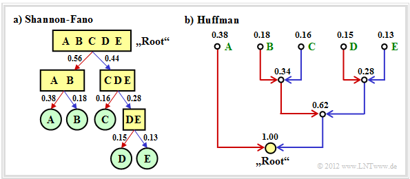
Tree structures according to Shannon-Fano and Huffman

The diagram shows the respective code trees for Shannon-Fano (left) and Huffman (right). The results can be summarised as follows:

The Shannon-Fano algorithm leads to the code

$\rm A$ → 11, $\rm B$ → 10, $\rm C$ → 01, $\rm D$ → 001, $\rm E$ → 000

and thus to the mean code word length

$$L_{\rm M} = (0.38 + 0.18 + 0.16) \cdot 2 + (0.15 + 0.13) \cdot 3 $$

$$\Rightarrow\hspace{0.3cm} L_{\rm M} = 2.28\,\,{\rm bit/source\hspace{0.15cm} symbol}\hspace{0.05cm}.$$

Using "Huffman", we get

$\rm A$ → 1, $\rm B$ → 001, $\rm C$ → 010, $\rm D$ → 001, $\rm E$ → 000

and a slightly smaller code word length:

$$L_{\rm M} = 0.38 \cdot 1 + (1-0.38) \cdot 3 $$

$$\Rightarrow\hspace{0.3cm} L_{\rm M} = 2.24\,\,{\rm bit/source\hspace{0.15cm} symbol}\hspace{0.05cm}. $$

There is no set of probabilities for which "Shannon–Fano" provides a better result than "Huffman", which always provides the best possible entropy encoder.
The graph also shows that the algorithms proceed in different directions in the tree diagram, namely once from the root to the individual symbols (Shannon–Fano), and secondly from the individual symbols to the root (Huffman).

The (German language) interactive applet "Huffman- und Shannon-Fano-Codierung ⇒ $\text{SWF}$ version" illustrates the procedure for two variants of entropy coding.

Arithmetic coding

Another form of entropy coding is arithmetic coding. Here, too, the symbol probabilities $p_μ$ must be known. For the index applies $μ = 1$, ... , $M$.

Here is a brief outline of the procedure:

In contrast to Huffman and Shannon-Fano coding, a symbol sequence of length $N$ is coded together in arithmetic coding. We write abbreviated $Q = 〈\hspace{0.05cm} q_1, q_2$, ... , $q_N \hspace{0.05cm} 〉$.
Each symbol sequence $Q_i$ is assigned a real number interval $I_i$ which is identified by the beginning $B_i$ and the interval width ${\it Δ}_i$ .
The "code" for the sequence $Q_i$ is the binary representation of a real number value from this interval: $r_i ∈ I_i = \big [B_i, B_i + {\it Δ}_i\big)$. This notation says that $B_i$ belongs to the interval $I_i$ (square bracket), but $B_i + {\it Δ}_i$ just does not (round bracket).
It is always $0 ≤ r_i < 1$. It makes sense to select $r_i$ from the interval $I_i$ in such a way that the value can be represented with as few bits as possible. However, there is always a minimum number of bits, which depends on the interval width ${\it Δ}_i$.

The algorithm for determining the interval parameters $B_i$ and ${\it Δ}_i$ is explained later in $\text{Example 4}$ , as is a decoding option.

First, there is a short example for the selection of the real number $r_i$ with regard to the minimum number of bits.
More detailed information on this can be found in the description of "Exercise 2.11Z".

$\text{Example 3:}$ For the two parameter sets of the arithmetic coding algorithm listed below, yields the following real results $r_i$ and the following codes belong to the associated interval $I_i$ :

$B_i = 0.25, {\it Δ}_i = 0.10 \ ⇒ \ I_i = \big[0.25, 0.35\big)\text{:}$

$$r_i = 0 \cdot 2^{-1} + 1 \cdot 2^{-2} = 0.25 \hspace{0.3cm}\Rightarrow\hspace{0.3cm} {\rm Code} \hspace{0.15cm} \boldsymbol{\rm 01} \in I_i \hspace{0.05cm},$$

$B_i = 0.65, {\it Δ}_i = 0.10 \ ⇒ \ I_i = \big[0.65, 0.75\big);$ note: $0.75$ does not belong to the interval:

$$r_i = 1 \cdot 2^{-1} + 0 \cdot 2^{-2} + 1 \cdot 2^{-3} + 1 \cdot 2^{-4} = 0.6875 \hspace{0.3cm}\Rightarrow\hspace{0.3cm} {\rm Code} \hspace{0.15cm} \boldsymbol{\rm 1011} \in I_i\hspace{0.05cm}. $$

However, to organise the sequential flow, one chooses the number of bits constant to $N_{\rm Bit} = \big\lceil {\rm log}_2 \hspace{0.15cm} ({1}/{\it \Delta_i})\big\rceil+1\hspace{0.05cm}. $

With the interval width ${\it Δ}_i = 0.10$ results $N_{\rm Bit} = 5$.
So the actual arithmetic codes would be 01000 and 10110 respectively.

$\text{Example 4:}$ Now let the symbol set size be $M = 3$ and let the symbols be denoted by $\rm X$, $\rm Y$ and $\rm Z$:

The character sequence $\rm XXYXZ$ ⇒ length of the source symbol sequence: $N = 5$.
Assume the probabilities $p_{\rm X} = 0.6$, $p_{\rm Y} = 0.2$ und $p_{\rm Z} = 0.2$.

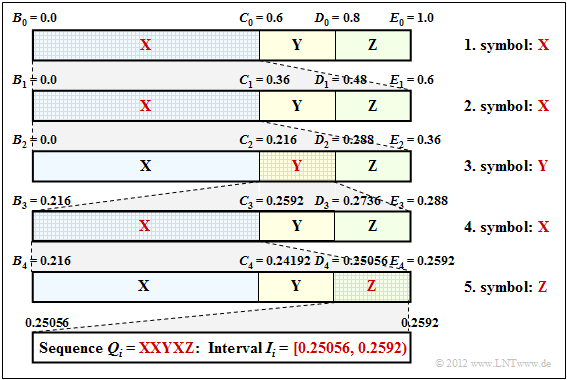
About the arithmetic coding algorithm

The diagram on the right shows the algorithm for determining the interval boundaries.

First, the entire probability range $($between $0$ and $1)$ is divided according to the symbol probabilities $p_{\rm X}$, $p_{\rm Y}$ and $p_{\rm Z}$ into three areas with the boundaries $B_0$, $C_0$, $D_0$ and $E_0$.
The first symbol present for coding is $\rm X$. Therefore, in the next step, the probability range from $B_1 = B_0 = 0$ to $E_1 = C_0 = 0.6$ is again divided in the ratio $0.6$ : $0.2$ : $0.2$.
After the second symbol $\rm X$ , the range limits are $B_2 = 0$, $C_2 = 0.216$, $D_2 = 0.288$ and $E_2 = 0.36$. Since the symbol $\rm Y$ is now pending, the range is subdivided between $0.216$ ... $0.288$.
After the fifth symbol $\rm Z$ , the interval $I_i$ for the considered symbol sequence $Q_i = \rm XXYXZ$ is fixed. A real number $r_i$ must now be found for which the following applies:: $0.25056 ≤ r_i < 0.2592$.
The only real number in the interval $I_i = \big[0.25056, 0.2592\big)$, that can be represented with seven bits is

$$r_i = 1 · 2^{–2} + 1 · 2^{–7} = 0.2578125.$$

Thus the coder output is fixed: 0100001.

Seven bits are therefore needed for these $N = 5$ symbols, exactly as many as with Huffman coding with the assignment $\rm X$ → 1, $\rm Y$ → 00, $\rm Z$ → 01.

However, arithmetic coding is superior to Huffman coding when the actual number of bits used in Huffman deviates even more from the optimal distribution, for example, when a character occurs extremely frequently.
Often, however, only the middle of the interval – in the example $0.25488$ – is represented in binary: 0.01000010011 .... The number of bits is obtained as follows:

$${\it Δ}_5 = 0.2592 - 0.25056 = 0.00864 \hspace{0.3cm}\Rightarrow \hspace{0.3cm}N_{\rm Bit} = \left\lceil {\rm log}_2 \hspace{0.15cm} \frac{1}{0.00864} \right\rceil + 1\hspace{0.15cm} = \left\lceil {\rm log}_2 \hspace{0.15cm} 115.7 \right\rceil + 1 = 8 \hspace{0.05cm}.$$

Thus the arithmetic code for this example with $N = 5$ input characters is: 01000010.

The decoding process can also be explained using the above graphic. The incoming bit sequence 0100001 is converted to $r = 0.2578125$ .
This lies in the first and second step respectively in the first area ⇒ symbol $\rm X$, in the third step in the second area ⇒ symbol $\rm Y$, and so on.

Further information on arithmetic coding can be found in $\text{WIKIPEDIA}$ and in [BCK02]^[1].

Run–Length coding

We consider a binary source $(M = 2)$ with the symbol set $\{$ $\rm A$, $\rm B$ $\}$, where one symbol occurs much more frequently than the other. For example, let $p_{\rm A} \gg p_{\rm B}$.

Entropy coding only makes sense here when applied to $k$–tuples.
A second possibility is »Run-length Coding« $\rm (RLC)$,
which considers the rarer character $\rm B$ as a separator and returns the lengths $L_i$ of the individual sub-strings $\rm AA\text{...}A$ as a result.

To illustrate the run-length coding

$\text{Example 5:}$ The graphic shows an example sequence

with the probabilities $p_{\rm A} = 0.9$ and $p_{\rm B} = 0.1$
⇒ source entropy $H = 0.469$ bit/source symbol.

The example sequence of length $N = 100$ contains the symbol $\rm B$ exactly ten times and the symbol $\rm A$ ninety times, i.e. the relative frequencies here correspond exactly to the probabilities.
You can see from this example:

The run-length coding of this sequence results in the sequence $ \langle \hspace{0.05cm}6, \ 14, \ 26, \ 11, \ 4, \ 10, \ 3,\ 9,\ 1,\ 16 \hspace{0.05cm} \rangle $.
If one represents the lengths $L_1$, ... , $L_{10}$ with five bits each, one thus requires $5 · 10 = 50$ bits.
The RLC data compression is thus not much worse than the theoretical limit that results according to the source entropy to $H · N ≈ 47$ bits.
The direct application of entropy coding would not result in any data compression here; rather, one continues to need $100$ bits.
Even with the formation of triples, $54$ bits would still be needed with Huffman, i.e. more than with run-length coding.

However, the example also shows two problems of run-length coding:

The lengths $L_i$ of the substrings are not limited. Special measures must be taken here if a length $L_i$ is greater than $2^5 = 32$ $($valid fo $N_{\rm Bit} = 5)$,
for example the variant »Run–Length Limited Coding« $\rm (RLLC)$. See also [Meck09]^[2] and "Exercise 2.13".
If the sequence does not end with $\rm B$ – which is rather the normal case with small probability $p_{\rm B}$ one must also provide special treatment for the end of the file.

Burrows–Wheeler transformation

To conclude this source coding chapter, we briefly discuss the algorithm published in 1994 by $\text{Michael Burrows}$ and $\text{David J. Wheeler}$ [BW94]^[3],

Example of the BWT (forward transformation)

which, although it has no compression potential on its own,
but it greatly improves the compression capability of other methods.

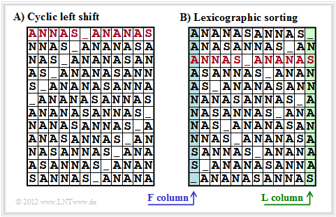
The Burrows–Wheeler Transformation accomplishes a blockwise sorting of data, which is illustrated in the diagram using the example of the text $\text{ANNAS_ANANAS}$ (meaning: Anna's pineapple) of length $N = 12$:

First, an $N×N$ matrix is generated from the string of length $N$ with each row resulting from the preceding row by cyclic left shift.
Then the BWT matrix is sorted lexicographically. The result of the transformation is the last column ⇒ $\text{L–Spalte}$. In the example, this results in $\text{_NSNNAANAAAS}$.
Furthermore, the primary index $I$ must also be passed on. This value indicates the row of the sorted BWT matrix that contains the original text (marked red in the graphic).
Of course, no matrix operations are necessary to determine the $\text{L–column}$ and the primary index. Rather, the BWT result can be found very quickly with pointer technology.

$\text{Furthermore, it should be noted about the BWT procedure:}$

Without an additional measure ⇒ a downstream „real compression” – the BWT does not lead to any data compression.
Rather, there is even a slight increase in the amount of data, since in addition to the $N$ characters, the primary index $I$ now also be transmitted.
For longer texts, however, this effect is negligible. Assuming 8 bit–ASCII–characters (one byte each) and the block length $N = 256$ the number of bytes per block only increases from $256$ to $257$, i.e. by only $0.4\%$.

We refer to the detailed descriptions of BWT in [Abel04]^[4].

Example for BWT (reverse transformation)

Finally, we will show how the original text can be reconstructed from the $\text{L}$–column (from "Last") of the BWT matrix.

For this, one still needs the primary index $I$, as well as the first column of the BWT matrix.
This $\text{F}$–column (from "First") does not have to be transferred, but results from the $\text{L}$–column very simply through lexicographic sorting.

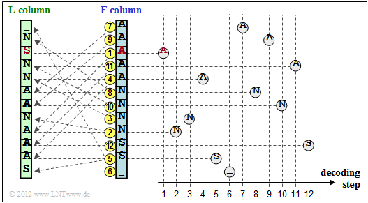
The graphic shows the reconstruction procedure for the example under consideration:

One starts in the line with the primary index $I$. The first character to be output is the $\rm A$ marked in red in the $\text{F}$–column. This step is marked in the graphic with a yellow (1).
This $\rm A$ is the third $\rm A$ character in the $\text{F}$–column. Now look for the third $\rm A$ in the $\text{L}$–column, find it in the line marked with (2) and output the corresponding N of the $\text{F}$–column.
The last N of the $\text{L}$–column is found in line (3). The character of the F column is output in the same line, i.e. an N again.

After $N = 12$ decoding steps, the reconstruction is completed.

$\text{Conclusion:}$

This example has shown that the Burrows–Wheeler transformation is nothing more than a sorting algorithm for texts. What is special about it is that the sorting is uniquely reversible.

This property and additionally its inner structure are the basis for compressing the BWT result by means of known and efficient methods such as $\text{Huffman}$ (a form of entropy coding) and $\text{run–length coding}$.

Application scenario for the Burrows-Wheeler transformation

As an example for embedding the $\text{Burrows–Wheeler Transformation}$ (BWT) into a chain of source coding methods, we choose a structure proposed in [Abel03]^[5]. We use the same text example $\text{ANNAS_ANANAS}$ as in the last section. The corresponding strings after each block are also given in the graphic.

Scheme for Burrows-Wheeler data compression

The $\rm BWT$ result is: $\text{_NSNNAANAAAS}$. BWT has not changed anything about the text length $N = 12$ but there are now four characters that are identical to their predecessors (highlighted in red in the graphic). In the original text, this was only the case once.
In the next block $\rm MTF$ ("Move–To–Front") , each input character from the set $\{$ $\rm A$, $\rm N$, $\rm S$, _$\}$ becomes an index $I ∈ \{0, 1, 2, 3\}$. However, this is not a simple mapping, but an algorithm given in "Exercise 1.13Z".
For our example, the MTF output sequence is $323303011002$, also with length $N = 12$. The four zeros in the MTF sequence (also in red font in the diagram) indicate that at each of these positions the BWT character is the same as its predecessor.
In large ASCII files, the frequency of the $0$ may well be more than $50\%$, while the other $255$ indices occur only rarely. Run-length coding $\rm (RCL)$ is an excellent way to compress such a text structure.
The block $\rm RCL0$ in the above coding chain denotes a special $\text{run-length coding}$ for zeros. The grey shading of the zeros indicates that a long zero sequence has been masked by a specific bit sequence (shorter than the zero sequence).
The entropy encoder $\rm (EC$, for example "Huffman"$)$ provides further compression. BWT and MTF only have the task in the coding chain of increasing the efficiency of "RLC0" and "EC" through character preprocessing. The output file is again binary.

Exercises for the chapter

Exercise 2.10: Shannon-Fano Coding

Exercise 2.11: Arithmetic Coding

Exercise 2.11Z: Arithmetic Coding once again

Exercise 2.12: Run–Length Coding and Run–Length Limited Coding

Exercise 2.13: Inverse Burrows-Wheeler Transformation

Exercise 2.13Z: Combination of BWT and MTF

References

↑ Bodden, E.; Clasen, M.; Kneis, J.: Algebraische Kodierung. Algebraic Coding. Proseminar, Chair of Computer Science IV, RWTH Aachen University, 2002.
↑ Mecking, M.: Information Theory. Lecture manuscript, Chair of Communications Engineering, Technical University of Munich, 2009.
↑ Burrows, M.; Wheeler, D.J.: A Block-sorting Lossless Data Compression Algorithm. Technical Report. Digital Equipment Corp. Communications, Palo Alto, 1994.
↑ Abel, J.: Grundlagen des Burrows-Wheeler-Kompressionsalgorithmus. In: Informatik Forschung & Entwicklung, no. 2, vol. 18, S. 80-87, Jan. 2004
↑ Abel, J.: Verlustlose Datenkompression auf Grundlage der Burrows-Wheeler-Transformation.
In: PIK - Praxis der Informationsverarbeitung und Kommunikation, no. 3, vol. 26, pp. 140-144, Sept. 2003.

[1] Bodden, E.; Clasen, M.; Kneis, J.: Algebraische Kodierung. Algebraic Coding. Proseminar, Chair of Computer Science IV, RWTH Aachen University, 2002.

[2] Mecking, M.: Information Theory. Lecture manuscript, Chair of Communications Engineering, Technical University of Munich, 2009.

[3] Burrows, M.; Wheeler, D.J.: A Block-sorting Lossless Data Compression Algorithm. Technical Report. Digital Equipment Corp. Communications, Palo Alto, 1994.

[4] Abel, J.: Grundlagen des Burrows-Wheeler-Kompressionsalgorithmus. In: Informatik Forschung & Entwicklung, no. 2, vol. 18, S. 80-87, Jan. 2004

[5] Abel, J.: Verlustlose Datenkompression auf Grundlage der Burrows-Wheeler-Transformation.
In: PIK - Praxis der Informationsverarbeitung und Kommunikation, no. 3, vol. 26, pp. 140-144, Sept. 2003.

[1]

[2]

[3]

[4]

[5]