Contents
ACF at the output of a non-recursive filter
We consider a non-recursive $M$–th order digital filter according to the following diagram.
The discrete-time input variable $〈\hspace{0.05cm}x_ν\hspace{0.05cm}〉$ is
- mean–free $(m_x = 0)$,
- Gaussian distributed (with standard deviation ⇒ "rms value" $σ_x)$, and
- without memory ("white noise") ⇒ statistically independent samples.
This results in the following properties:
- The discrete-time auto-correlation function $\rm (ACF)$ at the input is:
- $$\varphi _x ( {k \cdot T_{\rm A} } ) = \left\{ {\begin{array}{*{20}c} {\sigma _x ^2 } & {\rm{for}\quad {\it k} = 0,} \\ 0 & {\rm{for}\quad {\it k} \ne 0.} \\\end{array}} \right.$$
- The ACF of the discrete-time output sequence $〈\hspace{0.05cm}y_ν\hspace{0.05cm}〉$ is given as follows:
- $$\varphi _y ( {k \cdot T_{\rm A} } ) = \sigma _x ^2 \cdot \sum\limits_{\mu = 0}^{M - k} {a_\mu \cdot a_{\mu + k } } \quad {\rm{for}}\quad {\it k} = 0, 1,\,\text{...}\,,\,{\it M}.$$
- All ACF values with $k > M$ are zero, and all ACF values with $k < M$ are symmetric about $k = 0$:
- $$\varphi _y ( { - k \cdot T_{\rm A} } ) = \varphi _y ( {k \cdot T_{\rm A} } ).$$
$\text{Example 1:}$ If discrete-time white noise with standard deviation $σ_x = 2$ is present at the input of a first-order non-recursive filter $($filter coefficients $a_0 = 0.6$, $a_1 = 0.8),$ the discrete ACF values of the output signal are (all other ACF values are zero):
- $$\varphi _y (0) = \sigma _x ^2 \cdot ( {a_0 ^2 + a_1 ^2 }) = 4,$$
- $$\varphi _y ( { - T_{\rm A} } ) = \varphi _y ( {T_{\rm A} } ) = \sigma _x ^2 \cdot a_0 \cdot a_1 = 1.92.$$
The graphic can be interpreted as follows:
- Because of $a_0^2 + a_1^2 = 1$, the output signal $y(t)$ has exactly the same variance $σ_y^2 = φ_y(0) = 0.4$ as the input signal: $σ_x^2 = φ_x(0)$.
- Unlike the input sequence $〈\hspace{0.05cm}x_ν\hspace{0.05cm}〉$, the output sequence $〈\hspace{0.05cm}y_ν\hspace{0.05cm}〉$ has statistical bindings between adjacent samples.
Determining the coefficients
Now the following question is to be answered: How can the coefficients $a_0$, ... , $a_M$ of a $M$–th order non-recursive filter can be determined,
- if the desired ACF values $φ_y(0)$, ... ,s $φ_y(M · T_{\rm A})$ are given,s and
- outside the range from $-M · T_{\rm A}$ to $+M · T_{\rm A}$ all ACF values are to be zero.
For the rms value $σ_x = 1$, the following nonlinear system of equations is obtained, using $φ_k = φ_y(k · T_{\rm A})$ for simplicity of notation:
- $$\begin{align*}\varphi _0 & = \sum\limits_{\mu = 0}^M {a_\mu^2 ,}\\ \varphi _1 & = \sum\limits_{\mu = 0}^{M - 1} {a_\mu \cdot a_{\mu + 1} ,} \\ & ... &\\ \varphi _{M - 1} & = a_0 \cdot a_{M - 1} + a_1 \cdot a_M , \\ \varphi _M & = a_0 \cdot a_M .\end{align*}$$
$\text{Conclusion:}$
- Thus, for the $M + 1$ coefficients, one also obtains $M + 1$ independent equations.
- By successive elimination of the coefficients $a_1$, ... , $a_M$, finally a nonlinear equation of higher order remains for $a_0$.
$\text{Example 2:}$ We consider the following constellation:
- a recursive filter of first order ⇒ $M = 1$,
- a discrete-time input sequence $〈\hspace{0.05cm}x_ν\hspace{0.05cm}〉$ with mean $m_x =$ 0 and rms value $σ_x = 1$,
- desired ACF values of the sequence $〈\hspace{0.05cm}y_ν\hspace{0.05cm}〉$: $ φ_y(0) = φ_0 =0.58$, $φ_y(±T_{\rm A}) = φ_1 = 0.21$.
- Thus, the above system of equations is:
- $$\varphi _0 = a_0 ^2 + a_1 ^2 = 0.58,$$
- $$\varphi _1 = a_0 \cdot a_1 = 0.21.$$
- This leads to an equation of degree $4$,
- $$a_0 ^2 + \left( { { {0.21} }/{ {a_0 } } } \right)^2 = 0.58\quad \Rightarrow \quad a_0 ^4 - 0.58 \cdot a_0 ^2 + 0.21^2 = 0.$$
- A solution represents $a_0 = 0.7$. By inserting it into the second equation, we find $a_1 = 0.3$.
One recognizes from this example that already in the simplest case ⇒ $M = 1$ for $a_0$ a nonlinear determination equation of degree $4$ results.
Ambiguities in the determination of the coefficients
As the last example showed, with $M = 1$ the determination equation for $a_0$ is of degree $4$. At the same time, this means that there are also four sets of coefficients, all leading to the same ACF.
This is obvious for the following reasons:
- The coefficients $a_0$ and $a_1$ can change sign simultaneously without changing the system of equations.
- Replacing $a_0$ by $a_1$ and vice versa results in the same equation of determination.
- This operation corresponds to a mirroring and shifting of the impulse response.
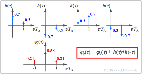
$\text{Example 3:}$ As shown in the last section, the parameter set $a_0 = 0.7$, $a_1 = 0.3$ is suitable to generate the ACF values $φ_0 = 0.58$ and $φ_1 = 0.21$. The desired ACF of the output sequence is then in detailed notation:
- $$\varphi_y(\tau) = 0.58 \cdot \delta(\tau) + 0.21 \cdot \delta(\tau - T_{\rm A}) + 0.21 \cdot \delta(\tau + T_{\rm A}) .$$
The same ACF is also obtained with the coefficients
- $a_0 = - 0.7,\quad a_1 = -0.3,$
- $a_0 = +0.3,\quad a_1 = +0.7,$
- $a_0 = - 0.3,\quad a_1 = -0.7.$
These configurations are obtained by
- simultaneously multiplying all coefficients by $-1$, and
- swapping the numerical values of $a_0$ and $a_1$.
The diagram shows the respective impulse responses leading to the desired ACF.
Exercises for the chapter
Exercise 5.5: ACF-equivalent Filters
Exercise 5.5Z: ACF after 1st Order Filter
Exercise 5.6: Filter Dimensioning
Exercise 5.6Z: Filter Dimensioning again


