Difference between revisions of "Applets:Capacity of Memoryless Digital Channels"
m (Text replacement - "Biographies_and_Bibliographies/LNTwww_members_from_LÜT#Tasn.C3.A1d_Kernetzky.2C_M.Sc._.28at_L.C3.9CT_since_2014.29" to "Biographies_and_Bibliographies/LNTwww_members_from_LÜT#Dr.-Ing._Tasn.C3.A1d_Kernetzky_.28at_L.C3.9CT_from_2014-2022.29") |
|||
| (47 intermediate revisions by 4 users not shown) | |||
| Line 1: | Line 1: | ||
| − | {{ | + | {{LntAppletLinkEnDe|transinformation_en|transinformation}} |
| + | |||
| − | == | + | ==Applet Description== |
<br> | <br> | ||
| − | In | + | In this applet, binary $(M=2)$ and ternary $(M=3)$ channel models without memory are considered with $M$ possible inputs $(X)$ and $M$ possible outputs $(Y)$. Such a channel is completely determined by the "probability mass function" $P_X(X)$ and the matrix $P_{\hspace{0.01cm}Y\hspace{0.03cm} \vert \hspace{0.01cm}X}(Y\hspace{0.03cm} \vert \hspace{0.03cm} X)$ of the "transition probabilities". |
| + | For these binary and ternary systems, the following information-theoretic descriptive quantities are derived and clarified: | ||
| + | *the "source entropy" $H(X)$ and the "sink entropy" $H(Y)$, | ||
| − | + | *the "equivocation" $H(X|Y)$ and the "irrelevance" $H(Y|X)$, | |
| − | + | ||
| − | * | + | *the "joint entropy" $H(XY)$ as well as the "mutual information" $I(X; Y)$, |
| − | * | + | |
| − | * | + | *the "channel capacity" as the decisive parameter of digital channel models without memory: |
:$$C = \max_{P_X(X)} \hspace{0.15cm} I(X;Y) \hspace{0.05cm}.$$ | :$$C = \max_{P_X(X)} \hspace{0.15cm} I(X;Y) \hspace{0.05cm}.$$ | ||
| − | + | These information-theoretical quantities can be calculated both in analytic–closed form or determined simulatively by evaluation of source and sink symbol sequence. | |
| − | == | + | ==Theoretical Background== |
<br> | <br> | ||
| − | === | + | ===Underlying model of digital signal transmission === |
| + | <br> | ||
| + | The set of possible »'''source symbols'''« is characterized by the discrete random variable $X$. | ||
| + | *In the binary case ⇒ $M_X= |X| = 2$ holds $X = \{\hspace{0.05cm}{\rm A}, \hspace{0.15cm} {\rm B} \hspace{0.05cm}\}$ with the probability mass function $($ $\rm PMF)$ $P_X(X)= \big (p_{\rm A},\hspace{0.15cm}p_{\rm B}\big)$ and the source symbol probabilities $p_{\rm A}$ and $p_{\rm B}=1- p_{\rm A}$. | ||
| − | + | *Accordingly, for a ternary source ⇒ $M_X= |X| = 3$: $X = \{\hspace{0.05cm}{\rm A}, \hspace{0.15cm} {\rm B}, \hspace{0.15cm} {\rm C} \hspace{0.05cm}\}$, $P_X(X)= \big (p_{\rm A},\hspace{0.15cm}p_{\rm B},\hspace{0.15cm}p_{\rm C}\big)$, $p_{\rm C}=1- p_{\rm A}-p_{\rm B}$. | |
| − | * | ||
| − | |||
| − | + | The set of possible »'''sink symbols'''« is characterized by the discrete random variable $Y$. These come from the same symbol set as the source symbols ⇒ $M_Y=M_X = M$. To simplify the following description, we denote them with lowercase letters, for example, for $M=3$: $Y = \{\hspace{0.05cm}{\rm a}, \hspace{0.15cm} {\rm b}, \hspace{0.15cm} {\rm c} \hspace{0.05cm}\}$. | |
| − | + | The relationship between the random variables $X$ and $Y$ is given by a »'''discrete memoryless channel model'''« $($ $\rm DMC)$. The left graph shows this for $M=2$ and the right graph for $M=3$. | |
| − | [[File:Transinf_1_neu.png|center|frame| | + | [[File:Transinf_1_neu.png|center|frame| $M=2$ (left) and for $M=3$ (right). <u>Please note:</u> In the right graph not all transitions are labeled]] |
| − | + | The following description applies to the simpler case $M=2$. For the calculation of all information theoretic quantities in the next section we need besides $P_X(X)$ and $P_Y(Y)$ the two-dimensional probability functions $($each a $2\times2$–matrix$)$ of all | |
| − | # [[Theory_of_Stochastic_Signals/ | + | # [[Theory_of_Stochastic_Signals/Statistical_Dependence_and_Independence#Conditional_probability|"conditional probabilities"]] ⇒ $P_{\hspace{0.01cm}Y\hspace{0.03cm} \vert \hspace{0.01cm}X}(Y\hspace{0.03cm} \vert \hspace{0.03cm} X)$ ⇒ given by the DMC model; |
| − | # [[Information_Theory/ | + | # [[Information_Theory/Some_Preliminary_Remarks_on_Two-Dimensional_Random_Variables#Joint_probability_and_joint_entropy|"joint probabilities"]] ⇒ $P_{XY}(X,\hspace{0.1cm}Y)$; |
| − | # [[Theory_of_Stochastic_Signals/ | + | # [[Theory_of_Stochastic_Signals/Statistical_Dependence_and_Independence#Inference_probability|"inference probabilities"]] ⇒ $P_{\hspace{0.01cm}X\hspace{0.03cm} \vert \hspace{0.03cm}Y}(X\hspace{0.03cm} \vert \hspace{0.03cm} Y)$. |
| − | |||
{{GraueBox|TEXT= | {{GraueBox|TEXT= | ||
| − | $\text{ | + | [[File:Transinf_2.png|right|frame|Considered model of the binary channel]] |
| − | * | + | $\text{Example 1}$: We consider the sketched binary channel. |
| + | * Let the falsification probabilities be: | ||
:$$\begin{align*}p_{\rm a\hspace{0.03cm}\vert \hspace{0.03cm}A} & = {\rm Pr}(Y\hspace{-0.1cm} = {\rm a}\hspace{0.05cm}\vert X \hspace{-0.1cm}= {\rm A}) = 0.95\hspace{0.05cm},\hspace{0.8cm}p_{\rm b\hspace{0.03cm}\vert \hspace{0.03cm}A} = {\rm Pr}(Y\hspace{-0.1cm} = {\rm b}\hspace{0.05cm}\vert X \hspace{-0.1cm}= {\rm A}) = 0.05\hspace{0.05cm},\\ | :$$\begin{align*}p_{\rm a\hspace{0.03cm}\vert \hspace{0.03cm}A} & = {\rm Pr}(Y\hspace{-0.1cm} = {\rm a}\hspace{0.05cm}\vert X \hspace{-0.1cm}= {\rm A}) = 0.95\hspace{0.05cm},\hspace{0.8cm}p_{\rm b\hspace{0.03cm}\vert \hspace{0.03cm}A} = {\rm Pr}(Y\hspace{-0.1cm} = {\rm b}\hspace{0.05cm}\vert X \hspace{-0.1cm}= {\rm A}) = 0.05\hspace{0.05cm},\\ | ||
| Line 50: | Line 54: | ||
\end{pmatrix} \hspace{0.05cm}.$$ | \end{pmatrix} \hspace{0.05cm}.$$ | ||
| − | * | + | *Furthermore, we assume source symbols that are not equally probable: |
:$$P_X(X) = \big ( p_{\rm A},\ p_{\rm B} \big )= | :$$P_X(X) = \big ( p_{\rm A},\ p_{\rm B} \big )= | ||
| Line 56: | Line 60: | ||
\hspace{0.05cm}.$$ | \hspace{0.05cm}.$$ | ||
| − | * | + | *Thus, for the probability function of the sink we get: |
:$$P_Y(Y) = \big [ {\rm Pr}( Y\hspace{-0.1cm} = {\rm a})\hspace{0.05cm}, \ {\rm Pr}( Y \hspace{-0.1cm}= {\rm b}) \big ] = \big ( 0.1\hspace{0.05cm},\ 0.9 \big ) \cdot | :$$P_Y(Y) = \big [ {\rm Pr}( Y\hspace{-0.1cm} = {\rm a})\hspace{0.05cm}, \ {\rm Pr}( Y \hspace{-0.1cm}= {\rm b}) \big ] = \big ( 0.1\hspace{0.05cm},\ 0.9 \big ) \cdot | ||
| Line 68: | Line 72: | ||
{\rm Pr}( Y \hspace{-0.1cm}= {\rm b}) = 1 - {\rm Pr}( Y \hspace{-0.1cm}= {\rm a}) = 0.545.$$ | {\rm Pr}( Y \hspace{-0.1cm}= {\rm b}) = 1 - {\rm Pr}( Y \hspace{-0.1cm}= {\rm a}) = 0.545.$$ | ||
| − | * | + | *The joint probabilities $p_{\mu \kappa} = \text{Pr}\big[(X = μ) ∩ (Y = κ)\big]$ between source and sink are: |
:$$\begin{align*}p_{\rm Aa} & = p_{\rm a} \cdot p_{\rm a\hspace{0.03cm}\vert \hspace{0.03cm}A} = 0.095\hspace{0.05cm},\hspace{0.5cm}p_{\rm Ab} = p_{\rm b} \cdot p_{\rm b\hspace{0.03cm}\vert \hspace{0.03cm}A} = 0.005\hspace{0.05cm},\\ | :$$\begin{align*}p_{\rm Aa} & = p_{\rm a} \cdot p_{\rm a\hspace{0.03cm}\vert \hspace{0.03cm}A} = 0.095\hspace{0.05cm},\hspace{0.5cm}p_{\rm Ab} = p_{\rm b} \cdot p_{\rm b\hspace{0.03cm}\vert \hspace{0.03cm}A} = 0.005\hspace{0.05cm},\\ | ||
| Line 81: | Line 85: | ||
\end{pmatrix} \hspace{0.05cm}.$$ | \end{pmatrix} \hspace{0.05cm}.$$ | ||
| − | * | + | * For the inference probabilities one obtains: |
:$$\begin{align*}p_{\rm A\hspace{0.03cm}\vert \hspace{0.03cm}a} & = p_{\rm Aa}/p_{\rm a} = 0.095/0.455 = 0.2088\hspace{0.05cm},\hspace{0.5cm}p_{\rm A\hspace{0.03cm}\vert \hspace{0.03cm}b} = p_{\rm Ab}/p_{\rm b} = 0.005/0.545 = 0.0092\hspace{0.05cm},\\ | :$$\begin{align*}p_{\rm A\hspace{0.03cm}\vert \hspace{0.03cm}a} & = p_{\rm Aa}/p_{\rm a} = 0.095/0.455 = 0.2088\hspace{0.05cm},\hspace{0.5cm}p_{\rm A\hspace{0.03cm}\vert \hspace{0.03cm}b} = p_{\rm Ab}/p_{\rm b} = 0.005/0.545 = 0.0092\hspace{0.05cm},\\ | ||
| Line 93: | Line 97: | ||
\end{pmatrix} \hspace{0.05cm}.$$ }} | \end{pmatrix} \hspace{0.05cm}.$$ }} | ||
<br clear=all><br><br> | <br clear=all><br><br> | ||
| − | ===Definition | + | ===Definition and interpretation of various entropy functions === |
| + | <br> | ||
| + | In the [[Information_Theory/Verschiedene_Entropien_zweidimensionaler_Zufallsgrößen|"theory section"]], all entropies relevant for two-dimensional random quantities are defined, which also apply to digital signal transmission. In addition, you will find two diagrams illustrating the relationship between the individual entropies. | ||
| + | *For digital signal transmission the right representation is appropriate, where the direction from source $X$ to the sink $Y$ is recognizable. | ||
| + | *We now interpret the individual information-theoretical quantities on the basis of this diagram. | ||
| − | |||
| − | |||
| − | |||
| + | [[File:EN_Inf_T_3_3_S2_vers2.png|EN_Inf_T_4_2_S2.png|center|frame|Two information-theoretic models for digital signal transmission. | ||
| + | <br> <u>Please note:</u> In the right graph $H_{XY}$ cannot be represented]] | ||
| − | + | *The »'''source entropy'''« $H(X)$ denotes the average information content of the source symbol sequence. With the symbol set size $|X|$ applies: | |
| − | |||
| − | |||
| − | |||
:$$H(X) = {\rm E} \left [ {\rm log}_2 \hspace{0.1cm} \frac{1}{P_X(X)}\right ] \hspace{0.1cm} | :$$H(X) = {\rm E} \left [ {\rm log}_2 \hspace{0.1cm} \frac{1}{P_X(X)}\right ] \hspace{0.1cm} | ||
| Line 110: | Line 114: | ||
P_X(x_{\mu}) \cdot {\rm log}_2 \hspace{0.1cm} \frac{1}{P_X(x_{\mu})} \hspace{0.05cm}.$$ | P_X(x_{\mu}) \cdot {\rm log}_2 \hspace{0.1cm} \frac{1}{P_X(x_{\mu})} \hspace{0.05cm}.$$ | ||
| − | * | + | *The »'''equivocation'''« $H(X|Y)$ indicates the average information content that an observer who knows exactly about the sink $Y$ gains by observing the source $X$ : |
:$$H(X|Y) = {\rm E} \left [ {\rm log}_2 \hspace{0.1cm} \frac{1}{P_{\hspace{0.05cm}X\hspace{-0.01cm}|\hspace{-0.01cm}Y}(X\hspace{-0.01cm} |\hspace{0.03cm} Y)}\right ] \hspace{0.2cm}=\hspace{0.2cm} \sum_{\mu = 1}^{|X|} \sum_{\kappa = 1}^{|Y|} | :$$H(X|Y) = {\rm E} \left [ {\rm log}_2 \hspace{0.1cm} \frac{1}{P_{\hspace{0.05cm}X\hspace{-0.01cm}|\hspace{-0.01cm}Y}(X\hspace{-0.01cm} |\hspace{0.03cm} Y)}\right ] \hspace{0.2cm}=\hspace{0.2cm} \sum_{\mu = 1}^{|X|} \sum_{\kappa = 1}^{|Y|} | ||
| Line 117: | Line 121: | ||
\hspace{0.05cm}.$$ | \hspace{0.05cm}.$$ | ||
| − | * | + | *The equivocation is the portion of the source entropy $H(X)$ that is lost due to channel interference (for digital channel: transmission errors). The »'''mutual information'''« $I(X; Y)$ remains, which reaches the sink: |
:$$I(X;Y) = {\rm E} \left [ {\rm log}_2 \hspace{0.1cm} \frac{P_{XY}(X, Y)}{P_X(X) \cdot P_Y(Y)}\right ] \hspace{0.2cm}=\hspace{0.2cm} \sum_{\mu = 1}^{|X|} \sum_{\kappa = 1}^{|Y|} | :$$I(X;Y) = {\rm E} \left [ {\rm log}_2 \hspace{0.1cm} \frac{P_{XY}(X, Y)}{P_X(X) \cdot P_Y(Y)}\right ] \hspace{0.2cm}=\hspace{0.2cm} \sum_{\mu = 1}^{|X|} \sum_{\kappa = 1}^{|Y|} | ||
| Line 123: | Line 127: | ||
\hspace{0.05cm} = H(X) - H(X|Y) \hspace{0.05cm}.$$ | \hspace{0.05cm} = H(X) - H(X|Y) \hspace{0.05cm}.$$ | ||
| − | * | + | *The »'''irrelevance'''« $H(Y|X)$ indicates the average information content that an observer who knows exactly about the source $X$ gains by observing the sink $Y$: |
:$$H(Y|X) = {\rm E} \left [ {\rm log}_2 \hspace{0.1cm} \frac{1}{P_{\hspace{0.05cm}Y\hspace{-0.01cm}|\hspace{-0.01cm}X}(Y\hspace{-0.01cm} |\hspace{0.03cm} X)}\right ] \hspace{0.2cm}=\hspace{0.2cm} \sum_{\mu = 1}^{|X|} \sum_{\kappa = 1}^{|Y|} | :$$H(Y|X) = {\rm E} \left [ {\rm log}_2 \hspace{0.1cm} \frac{1}{P_{\hspace{0.05cm}Y\hspace{-0.01cm}|\hspace{-0.01cm}X}(Y\hspace{-0.01cm} |\hspace{0.03cm} X)}\right ] \hspace{0.2cm}=\hspace{0.2cm} \sum_{\mu = 1}^{|X|} \sum_{\kappa = 1}^{|Y|} | ||
| Line 130: | Line 134: | ||
\hspace{0.05cm}.$$ | \hspace{0.05cm}.$$ | ||
| − | * | + | *The »'''sink entropy'''« $H(Y)$, the mean information content of the sink. $H(Y)$ is the sum of the useful mutual information $I(X; Y)$ and the useless irrelevance $H(Y|X)$, which comes exclusively from channel errors: |
:$$H(Y) = {\rm E} \left [ {\rm log}_2 \hspace{0.1cm} \frac{1}{P_Y(Y)}\right ] \hspace{0.1cm} | :$$H(Y) = {\rm E} \left [ {\rm log}_2 \hspace{0.1cm} \frac{1}{P_Y(Y)}\right ] \hspace{0.1cm} | ||
| Line 136: | Line 140: | ||
\hspace{0.05cm}.$$ | \hspace{0.05cm}.$$ | ||
| − | * | + | *The »'''joint entropy'''« $H(XY)$ is the average information content of the 2D random quantity $XY$. It also describes an upper bound for the sum of source entropy and sink entropy: |
:$$H(XY) = {\rm E} \left [ {\rm log} \hspace{0.1cm} \frac{1}{P_{XY}(X, Y)}\right ] = \sum_{\mu = 1}^{|X|} \hspace{0.1cm} \sum_{\kappa = 1}^{|Y|} \hspace{0.1cm} | :$$H(XY) = {\rm E} \left [ {\rm log} \hspace{0.1cm} \frac{1}{P_{XY}(X, Y)}\right ] = \sum_{\mu = 1}^{|X|} \hspace{0.1cm} \sum_{\kappa = 1}^{|Y|} \hspace{0.1cm} | ||
P_{XY}(x_{\mu}\hspace{0.05cm}, y_{\kappa}) \cdot {\rm log} \hspace{0.1cm} \frac{1}{P_{XY}(x_{\mu}\hspace{0.05cm}, y_{\kappa})}\le H(X) + H(Y) \hspace{0.05cm}.$$ | P_{XY}(x_{\mu}\hspace{0.05cm}, y_{\kappa}) \cdot {\rm log} \hspace{0.1cm} \frac{1}{P_{XY}(x_{\mu}\hspace{0.05cm}, y_{\kappa})}\le H(X) + H(Y) \hspace{0.05cm}.$$ | ||
| − | + | ||
{{GraueBox|TEXT= | {{GraueBox|TEXT= | ||
| − | $\text{ | + | [[File:Transinf_2.png|right|frame|Considered model of the binary channel]] |
| + | $\text{Example 2}$: The same requirements as for [[Applets:Capacity_of_Memoryless_Digital_Channels#Underlying_model_of_digital_signal_transmission|$\text{Example 1}$]] apply: | ||
| − | '''(1)''' | + | '''(1)''' The source symbols are not equally probable: |
:$$P_X(X) = \big ( p_{\rm A},\ p_{\rm B} \big )= | :$$P_X(X) = \big ( p_{\rm A},\ p_{\rm B} \big )= | ||
\big ( 0.1,\ 0.9 \big ) | \big ( 0.1,\ 0.9 \big ) | ||
\hspace{0.05cm}.$$ | \hspace{0.05cm}.$$ | ||
| − | '''(2)''' | + | '''(2)''' Let the falsification probabilities be: |
:$$\begin{align*}p_{\rm a\hspace{0.03cm}\vert \hspace{0.03cm}A} & = {\rm Pr}(Y\hspace{-0.1cm} = {\rm a}\hspace{0.05cm}\vert X \hspace{-0.1cm}= {\rm A}) = 0.95\hspace{0.05cm},\hspace{0.8cm}p_{\rm b\hspace{0.03cm}\vert \hspace{0.03cm}A} = {\rm Pr}(Y\hspace{-0.1cm} = {\rm b}\hspace{0.05cm}\vert X \hspace{-0.1cm}= {\rm A}) = 0.05\hspace{0.05cm},\\ | :$$\begin{align*}p_{\rm a\hspace{0.03cm}\vert \hspace{0.03cm}A} & = {\rm Pr}(Y\hspace{-0.1cm} = {\rm a}\hspace{0.05cm}\vert X \hspace{-0.1cm}= {\rm A}) = 0.95\hspace{0.05cm},\hspace{0.8cm}p_{\rm b\hspace{0.03cm}\vert \hspace{0.03cm}A} = {\rm Pr}(Y\hspace{-0.1cm} = {\rm b}\hspace{0.05cm}\vert X \hspace{-0.1cm}= {\rm A}) = 0.05\hspace{0.05cm},\\ | ||
p_{\rm a\hspace{0.03cm}\vert \hspace{0.03cm}B} & = {\rm Pr}(Y\hspace{-0.1cm} = {\rm a}\hspace{0.05cm}\vert X \hspace{-0.1cm}= {\rm B}) = 0.40\hspace{0.05cm},\hspace{0.8cm}p_{\rm b\hspace{0.03cm}\vert \hspace{0.03cm}B} = {\rm Pr}(Y\hspace{-0.1cm} = {\rm b}\hspace{0.05cm}\vert X \hspace{-0.1cm}= {\rm B}) = 0.60\end{align*}$$ | p_{\rm a\hspace{0.03cm}\vert \hspace{0.03cm}B} & = {\rm Pr}(Y\hspace{-0.1cm} = {\rm a}\hspace{0.05cm}\vert X \hspace{-0.1cm}= {\rm B}) = 0.40\hspace{0.05cm},\hspace{0.8cm}p_{\rm b\hspace{0.03cm}\vert \hspace{0.03cm}B} = {\rm Pr}(Y\hspace{-0.1cm} = {\rm b}\hspace{0.05cm}\vert X \hspace{-0.1cm}= {\rm B}) = 0.60\end{align*}$$ | ||
| Line 159: | Line 164: | ||
\end{pmatrix} \hspace{0.05cm}.$$ | \end{pmatrix} \hspace{0.05cm}.$$ | ||
| − | [[File:Inf_T_1_1_S4_vers2.png|frame| | + | [[File:Inf_T_1_1_S4_vers2.png|frame|Binary entropy function as a function of $p$|right]] |
| − | * | + | *Because of condition '''(1)''' we obtain for the source entropy with the [[Information_Theory/Discrete_Memoryless_Sources#Binary_entropy_function|"binary entropy function"]] $H_{\rm bin}(p)$: |
:$$H(X) = p_{\rm A} \cdot {\rm log_2}\hspace{0.1cm}\frac{1}{\hspace{0.1cm}p_{\rm A}\hspace{0.1cm} } + p_{\rm B} \cdot {\rm log_2}\hspace{0.1cm}\frac{1}{p_{\rm B} }= H_{\rm bin} (p_{\rm A}) = H_{\rm bin} (0.1)= 0.469 \ {\rm bit} | :$$H(X) = p_{\rm A} \cdot {\rm log_2}\hspace{0.1cm}\frac{1}{\hspace{0.1cm}p_{\rm A}\hspace{0.1cm} } + p_{\rm B} \cdot {\rm log_2}\hspace{0.1cm}\frac{1}{p_{\rm B} }= H_{\rm bin} (p_{\rm A}) = H_{\rm bin} (0.1)= 0.469 \ {\rm bit} | ||
\hspace{0.05cm};$$ | \hspace{0.05cm};$$ | ||
| − | ::$$H_{\rm bin} (p) = p \cdot {\rm log_2}\hspace{0.1cm}\frac{1}{\hspace{0.1cm}p\hspace{0.1cm} } + (1 - p) \cdot {\rm log_2}\hspace{0.1cm}\frac{1}{1 - p} \hspace{0.5cm}{\rm ( | + | ::$$H_{\rm bin} (p) = p \cdot {\rm log_2}\hspace{0.1cm}\frac{1}{\hspace{0.1cm}p\hspace{0.1cm} } + (1 - p) \cdot {\rm log_2}\hspace{0.1cm}\frac{1}{1 - p} \hspace{0.5cm}{\rm (unit\hspace{-0.15cm}: \hspace{0.15cm}bit\hspace{0.15cm}or\hspace{0.15cm}bit/symbol)} |
\hspace{0.05cm}.$$ | \hspace{0.05cm}.$$ | ||
| − | * | + | * Correspondingly, for the sink entropy with PMF $P_Y(Y) = \big ( p_{\rm a},\ p_{\rm b} \big )= |
\big ( 0.455,\ 0.545 \big )$: | \big ( 0.455,\ 0.545 \big )$: | ||
:$$H(Y) = H_{\rm bin} (0.455)= 0.994 \ {\rm bit} | :$$H(Y) = H_{\rm bin} (0.455)= 0.994 \ {\rm bit} | ||
\hspace{0.05cm}.$$ | \hspace{0.05cm}.$$ | ||
| − | * | + | *Next, we calculate the joint entropy: |
:$$H(XY) = p_{\rm Aa} \cdot {\rm log_2}\hspace{0.1cm}\frac{1}{\hspace{0.1cm}p_{\rm Aa}\hspace{0.1cm} }+ p_{\rm Ab} \cdot {\rm log_2}\hspace{0.1cm}\frac{1}{\hspace{0.1cm}p_{\rm Ab}\hspace{0.1cm} }+p_{\rm Ba} \cdot {\rm log_2}\hspace{0.1cm}\frac{1}{\hspace{0.1cm}p_{\rm Ba}\hspace{0.1cm} }+ p_{\rm Bb} \cdot {\rm log_2}\hspace{0.1cm}\frac{1}{\hspace{0.1cm}p_{\rm Bb}\hspace{0.1cm} }$$ | :$$H(XY) = p_{\rm Aa} \cdot {\rm log_2}\hspace{0.1cm}\frac{1}{\hspace{0.1cm}p_{\rm Aa}\hspace{0.1cm} }+ p_{\rm Ab} \cdot {\rm log_2}\hspace{0.1cm}\frac{1}{\hspace{0.1cm}p_{\rm Ab}\hspace{0.1cm} }+p_{\rm Ba} \cdot {\rm log_2}\hspace{0.1cm}\frac{1}{\hspace{0.1cm}p_{\rm Ba}\hspace{0.1cm} }+ p_{\rm Bb} \cdot {\rm log_2}\hspace{0.1cm}\frac{1}{\hspace{0.1cm}p_{\rm Bb}\hspace{0.1cm} }$$ | ||
:$$\Rightarrow \hspace{0.3cm}H(XY) = 0.095 \cdot {\rm log_2}\hspace{0.1cm}\frac{1}{0.095 } +0.005 \cdot {\rm log_2}\hspace{0.1cm}\frac{1}{0.005 }+0.36 \cdot {\rm log_2}\hspace{0.1cm}\frac{1}{0.36 }+0.54 \cdot {\rm log_2}\hspace{0.1cm}\frac{1}{0.54 }= 1.371 \ {\rm bit} | :$$\Rightarrow \hspace{0.3cm}H(XY) = 0.095 \cdot {\rm log_2}\hspace{0.1cm}\frac{1}{0.095 } +0.005 \cdot {\rm log_2}\hspace{0.1cm}\frac{1}{0.005 }+0.36 \cdot {\rm log_2}\hspace{0.1cm}\frac{1}{0.36 }+0.54 \cdot {\rm log_2}\hspace{0.1cm}\frac{1}{0.54 }= 1.371 \ {\rm bit} | ||
\hspace{0.05cm}.$$ | \hspace{0.05cm}.$$ | ||
| − | + | According to the upper left diagram, the remaining information-theoretic quantities are thus also computable: | |
| − | [[File:Transinf_4.png|right|frame| | + | [[File:Transinf_4.png|right|frame|Information-theoretic model for $\text{Example 2}$]] |
| − | * | + | *the »'''equivocation'''«: |
:$$H(X \vert Y) \hspace{-0.01cm} =\hspace{-0.01cm} H(XY) \hspace{-0.01cm} -\hspace{-0.01cm} H(Y) \hspace{-0.01cm} = \hspace{-0.01cm} 1.371\hspace{-0.01cm} -\hspace{-0.01cm} 0.994\hspace{-0.01cm} =\hspace{-0.01cm} 0.377\ {\rm bit} | :$$H(X \vert Y) \hspace{-0.01cm} =\hspace{-0.01cm} H(XY) \hspace{-0.01cm} -\hspace{-0.01cm} H(Y) \hspace{-0.01cm} = \hspace{-0.01cm} 1.371\hspace{-0.01cm} -\hspace{-0.01cm} 0.994\hspace{-0.01cm} =\hspace{-0.01cm} 0.377\ {\rm bit} | ||
\hspace{0.05cm},$$ | \hspace{0.05cm},$$ | ||
| − | * | + | *the »'''irrelevance'''«: |
:$$H(Y \vert X) = H(XY) - H(X) = 1.371 - 0.994 = 0.902\ {\rm bit} | :$$H(Y \vert X) = H(XY) - H(X) = 1.371 - 0.994 = 0.902\ {\rm bit} | ||
\hspace{0.05cm}.$$ | \hspace{0.05cm}.$$ | ||
| − | * | + | *the »'''mutual information'''« : |
:$$I(X;Y) = H(X) + H(Y) - H(XY) = 0.469 + 0.994 - 1.371 = 0.092\ {\rm bit} | :$$I(X;Y) = H(X) + H(Y) - H(XY) = 0.469 + 0.994 - 1.371 = 0.092\ {\rm bit} | ||
\hspace{0.05cm},$$ | \hspace{0.05cm},$$ | ||
| − | + | The results are summarized in the graph. | |
| − | + | <u>Note</u>: Equivocation and irrelevance could also be computed (but with extra effort) directly from the corresponding probability functions, for example: | |
:$$H(Y \vert X) = \hspace{-0.2cm} \sum_{(x, y) \hspace{0.05cm}\in \hspace{0.05cm}XY} \hspace{-0.2cm} P_{XY}(x,\hspace{0.05cm}y) \cdot {\rm log}_2 \hspace{0.1cm} \frac{1}{P_{\hspace{0.05cm}Y\hspace{-0.01cm}\vert \hspace{0.03cm}X} | :$$H(Y \vert X) = \hspace{-0.2cm} \sum_{(x, y) \hspace{0.05cm}\in \hspace{0.05cm}XY} \hspace{-0.2cm} P_{XY}(x,\hspace{0.05cm}y) \cdot {\rm log}_2 \hspace{0.1cm} \frac{1}{P_{\hspace{0.05cm}Y\hspace{-0.01cm}\vert \hspace{0.03cm}X} | ||
| Line 206: | Line 211: | ||
| − | |||
{{GraueBox|TEXT= | {{GraueBox|TEXT= | ||
| − | $\text{ | + | [[File:Transinf_3.png|right|frame|Considered model of the ternary channel:<br> Red transitions represent $p_{\rm a\hspace{0.03cm}\vert \hspace{0.03cm}A} = p_{\rm b\hspace{0.03cm}\vert \hspace{0.03cm}B} = p_{\rm c\hspace{0.03cm}\vert \hspace{0.03cm}C} = q$ and<br> blue ones for $p_{\rm b\hspace{0.03cm}\vert \hspace{0.03cm}A} = p_{\rm c\hspace{0.03cm}\vert \hspace{0.03cm}A} =\text{...}= p_{\rm b\hspace{0.03cm}\vert \hspace{0.03cm}C}= (1-q)/2$]] |
| + | $\text{Example 3}$: Now we consider a transmission system with $M_X = M_Y = M=3$. | ||
| − | '''(1)''' | + | '''(1)''' Let the source symbols be equally probable: |
:$$P_X(X) = \big ( p_{\rm A},\ p_{\rm B},\ p_{\rm C} \big )= | :$$P_X(X) = \big ( p_{\rm A},\ p_{\rm B},\ p_{\rm C} \big )= | ||
\big ( 1/3,\ 1/3,\ 1/3 \big )\hspace{0.30cm}\Rightarrow\hspace{0.30cm}H(X)={\rm log_2}\hspace{0.1cm}3 \approx 1.585 \ {\rm bit} | \big ( 1/3,\ 1/3,\ 1/3 \big )\hspace{0.30cm}\Rightarrow\hspace{0.30cm}H(X)={\rm log_2}\hspace{0.1cm}3 \approx 1.585 \ {\rm bit} | ||
\hspace{0.05cm}.$$ | \hspace{0.05cm}.$$ | ||
| − | '''(2)''' | + | '''(2)''' The channel model is symmetric ⇒ the sink symbols are also equally probable: |
:$$P_Y(Y) = \big ( p_{\rm a},\ p_{\rm b},\ p_{\rm c} \big )= | :$$P_Y(Y) = \big ( p_{\rm a},\ p_{\rm b},\ p_{\rm c} \big )= | ||
\big ( 1/3,\ 1/3,\ 1/3 \big )\hspace{0.30cm}\Rightarrow\hspace{0.30cm}H(Y)={\rm log_2}\hspace{0.1cm}3 \approx 1.585 \ {\rm bit} | \big ( 1/3,\ 1/3,\ 1/3 \big )\hspace{0.30cm}\Rightarrow\hspace{0.30cm}H(Y)={\rm log_2}\hspace{0.1cm}3 \approx 1.585 \ {\rm bit} | ||
\hspace{0.05cm}.$$ | \hspace{0.05cm}.$$ | ||
| − | '''(3)''' | + | '''(3)''' The joint probabilities are obtained as follows: |
:$$p_{\rm Aa}= p_{\rm Bb}= p_{\rm Cc}= q/M,$$ | :$$p_{\rm Aa}= p_{\rm Bb}= p_{\rm Cc}= q/M,$$ | ||
:$$p_{\rm Ab}= p_{\rm Ac}= p_{\rm Ba}= p_{\rm Bc} = p_{\rm Ca}= p_{\rm Cb} = (1-q)/(2M)$$ | :$$p_{\rm Ab}= p_{\rm Ac}= p_{\rm Ba}= p_{\rm Bc} = p_{\rm Ca}= p_{\rm Cb} = (1-q)/(2M)$$ | ||
:$$\Rightarrow\hspace{0.30cm}H(XY) = 3 \cdot p_{\rm Aa} \cdot {\rm log_2}\hspace{0.1cm}\frac{1}{\hspace{0.1cm}p_{\rm Aa}\hspace{0.1cm} }+6 \cdot p_{\rm Ab} \cdot {\rm log_2}\hspace{0.1cm}\frac{1}{\hspace{0.1cm}p_{\rm Ab}\hspace{0.1cm} }= \ | :$$\Rightarrow\hspace{0.30cm}H(XY) = 3 \cdot p_{\rm Aa} \cdot {\rm log_2}\hspace{0.1cm}\frac{1}{\hspace{0.1cm}p_{\rm Aa}\hspace{0.1cm} }+6 \cdot p_{\rm Ab} \cdot {\rm log_2}\hspace{0.1cm}\frac{1}{\hspace{0.1cm}p_{\rm Ab}\hspace{0.1cm} }= \ | ||
\text{...} \ = q \cdot {\rm log_2}\hspace{0.1cm}\frac{M}{q }+ (1-q) \cdot {\rm log_2}\hspace{0.1cm}\frac{M}{(1-q)/2 }.$$ | \text{...} \ = q \cdot {\rm log_2}\hspace{0.1cm}\frac{M}{q }+ (1-q) \cdot {\rm log_2}\hspace{0.1cm}\frac{M}{(1-q)/2 }.$$ | ||
| − | [[File:Transinf_10.png|right|frame| | + | [[File:Transinf_10.png|right|frame|Some results for $\text{Example 3}$]] |
| − | '''(4)''' | + | '''(4)''' For the mutual information we get after some transformations considering the equation |
:$$I(X;Y) = H(X) + H(Y) - H(XY)\text{:}$$ | :$$I(X;Y) = H(X) + H(Y) - H(XY)\text{:}$$ | ||
:$$\Rightarrow \hspace{0.3cm} I(X;Y) = {\rm log_2}\ (M) - (1-q) -H_{\rm bin}(q).$$ | :$$\Rightarrow \hspace{0.3cm} I(X;Y) = {\rm log_2}\ (M) - (1-q) -H_{\rm bin}(q).$$ | ||
| − | * | + | * For error-free ternary transfer $(q=1)$ holds $I(X;Y) = H(X) = H(Y)={\rm log_2}\hspace{0.1cm}3$. |
| − | * | + | |
| − | * | + | * With $q=0.8$ the mutual information already decreases to $I(X;Y) = 0.663$, with $q=0.5$ to $0.085$ bit. |
| − | * | + | |
| − | * | + | *The worst case from the point of view of information theory is $q=1/3$ ⇒ $I(X;Y) = 0$. |
| + | |||
| + | *On the other hand, the worst case from the point of view of transmission theory is $q=0$ ⇒ "not a single transmission symbol arrives correctly" is not so bad from the point of view of information theory. | ||
| + | |||
| + | * In order to be able to use this good result, however, channel coding is required at the transmitting end. }} | ||
<br><br> | <br><br> | ||
| − | ===Definition | + | ===Definition and meaning of channel capacity === |
| − | + | <br> | |
| − | + | If one calculates the mutual information $I(X, Y)$ as explained in $\text{Example 2}$, then this depends not only on the discrete memoryless channel $\rm (DMC)$, but also on the source statistic ⇒ $P_X(X)$. Ergo: '''The mutual information''' $I(X, Y)$ ''' is not a pure channel characteristic'''. | |
{{BlaueBox|TEXT= | {{BlaueBox|TEXT= | ||
| − | $\text{Definition:}$ | + | $\text{Definition:}$ The »'''channel capacity'''« introduced by [https://en.wikipedia.org/wiki/Claude_Shannon $\text{Claude E. Shannon}$] according to his standard work [Sha48]<ref name = ''Sha48''>Shannon, C.E.: A Mathematical Theory of Communication.[[File:Transinf_1_neu.png|center|frame| $M=2$ (left) and for $M=3$ (right). <u>Please note:</u> In the right graph not all transitions are labeled]] In: Bell Syst. Techn. J. 27 (1948), S. 379-423 und S. 623-656.</ref>: |
:$$C = \max_{P_X(X)} \hspace{0.15cm} I(X;Y) \hspace{0.05cm}.$$ | :$$C = \max_{P_X(X)} \hspace{0.15cm} I(X;Y) \hspace{0.05cm}.$$ | ||
| − | + | *The additional unit "bit/use" is often added. Since according to this definition the best possible source statistics are always the basis: | |
| + | :⇒ $C$ depends only on the channel properties ⇒ $P_{Y \vert X}(Y \vert X)$ but not on the source statistics ⇒ $P_X(X)$. }} | ||
| − | Shannon | + | |
| + | Shannon needed the quantity $C$ to formulate the "Channel Coding Theorem" – one of the highlights of the information theory he founded. | ||
{{BlaueBox|TEXT= | {{BlaueBox|TEXT= | ||
| − | $\text{ | + | $\text{Shannon's Channel Coding Theorem:}$ |
| − | * | + | *For every transmission channel with channel capacity $C > 0$, there exists $($at least$)$ one $(k,\ n)$ block code, whose $($block$)$ error probability approaches zero as long as the code rate $R = k/n$ is less than or equal to the channel capacity: |
| − | * | + | :$$R ≤ C.$$ |
| + | * The prerequisite for this, however, is that the following applies to the block length of this code: | ||
| + | :$$n → ∞.$$ | ||
| + | $\text{Reverse of Shannon's channel coding theorem:}$ | ||
| + | |||
| + | :If the rate $R$ of the $(n$, $k)$ block code used is larger than the channel capacity $C$, then an arbitrarily small block error probability can never be achieved.}} | ||
| − | |||
| − | |||
| − | |||
| − | |||
{{GraueBox|TEXT= | {{GraueBox|TEXT= | ||
| − | $\ | + | [[File:Transinf_9.png|right|frame|Information-theoretic quantities for <br>different $p_{\rm A}$ and $p_{\rm B}= 1- p_{\rm A}$ ]] |
| − | + | $\text{Example 4}$: We consider the same discrete memoryless channel as in $\text{Example 2}$. | |
| + | *The symbol probabilities $p_{\rm A} = 0.1$ and $p_{\rm B}= 1- p_{\rm A}=0.9$ were assumed. | ||
| + | |||
| + | *The mutual information is $I(X;Y)= 0.092$ bit/channel use ⇒ first row, see fourth column in the table. | ||
| − | |||
| − | |||
| − | + | The »'''channel capacity'''« is the mutual information $I(X, Y)$ with best possible symbol probabilities<br> $p_{\rm A} = 0.55$ and $p_{\rm B}= 1- p_{\rm A}=0.45$: | |
| − | + | :$$C = \max_{P_X(X)} \hspace{0.15cm} I(X;Y) = 0.284 \ \rm bit/channel \hspace{0.05cm} access \hspace{0.05cm}.$$ | |
| − | |||
| − | |||
| + | From the table you can see further $($we do without the additional unit "bit/channel use" in the following$)$: | ||
| + | #The parameter $p_{\rm A} = 0.1$ was chosen very unfavorably, because with the present channel the symbol $\rm A$ is more falsified than $\rm B$. | ||
| + | #Already with $p_{\rm A} = 0.9$ the mutual information results in a somewhat better value: $I(X; Y)=0.130$. | ||
| + | #For the same reason $p_{\rm A} = 0.55$, $p_{\rm B} = 0.45$ gives a slightly better result than equally probable symbols $(p_{\rm A} = p_{\rm B} =0.5)$. | ||
| + | #The more asymmetric the channel is, the more the optimal probability function $P_X(X)$ deviates from the uniform distribution. Conversely: If the channel is symmetric, the uniform distribution is always obtained.}} | ||
| − | + | ||
| + | The ternary channel of $\text{Example 3}$ is symmetric. Therefore here $P_X(X) = \big ( 1/3,\ 1/3,\ 1/3 \big )$ is optimal for each $q$–value, and the mutual information $I(X;Y)$ given in the result table is at the same time the channel capacity $C$. | ||
| Line 278: | Line 295: | ||
==Exercises== | ==Exercises== | ||
| − | + | <br> | |
*First, select the number $(1,\ 2, \text{...} \ )$ of the task to be processed. The number "$0$" corresponds to a "Reset": Same setting as at program start. | *First, select the number $(1,\ 2, \text{...} \ )$ of the task to be processed. The number "$0$" corresponds to a "Reset": Same setting as at program start. | ||
*A task description is displayed. The parameter values are adjusted. Solution after pressing "Show Solution". | *A task description is displayed. The parameter values are adjusted. Solution after pressing "Show Solution". | ||
| + | *Source symbols are denoted by uppercase letters (binary: $\rm A$, $\rm B$), sink symbols by lowercase letters ($\rm a$, $\rm b$). Error-free transmission: $\rm A \rightarrow a$. | ||
*For all entropy values, the unit "bit/use" would have to be added. | *For all entropy values, the unit "bit/use" would have to be added. | ||
| − | |||
| − | |||
| − | |||
| − | |||
| − | |||
| − | |||
| − | |||
{{BlueBox|TEXT= | {{BlueBox|TEXT= | ||
'''(1)''' Let $p_{\rm A} = p_{\rm B} = 0.5$ and $p_{\rm b \vert A} = p_{\rm a \vert B} = 0.1$. What is the channel model? What are the entropies $H(X), \, H(Y)$ and the mutual information $I(X;\, Y)$?}} | '''(1)''' Let $p_{\rm A} = p_{\rm B} = 0.5$ and $p_{\rm b \vert A} = p_{\rm a \vert B} = 0.1$. What is the channel model? What are the entropies $H(X), \, H(Y)$ and the mutual information $I(X;\, Y)$?}} | ||
| − | :* Considered is the BSC model (Binary Symmetric Channel). Because of $p_{\rm A} = p_{\rm B} = 0.5$ holds for the entropies: $H(X) = H(Y) = 1$. | + | :* Considered is the BSC model (Binary Symmetric Channel). Because of $p_{\rm A} = p_{\rm B} = 0.5$ it holds for the entropies: $H(X) = H(Y) = 1$. |
:* Because of $p_{\rm b \vert A} = p_{\rm a \vert B} = 0.1$ eqivocation and irrelevance are also equal: $H(X \vert Y) = H(Y \vert X) = H_{\rm bin}(p_{\rm b \vert A}) = H_{\rm bin}(0.1) =0.469$. | :* Because of $p_{\rm b \vert A} = p_{\rm a \vert B} = 0.1$ eqivocation and irrelevance are also equal: $H(X \vert Y) = H(Y \vert X) = H_{\rm bin}(p_{\rm b \vert A}) = H_{\rm bin}(0.1) =0.469$. | ||
:* The mutual information is $I(X;\, Y) = H(X) - H(X \vert Y)= 1-H_{\rm bin}(p_{\rm b \vert A}) = 0.531$ and the joint entropy is $H(XY) =1.469$. | :* The mutual information is $I(X;\, Y) = H(X) - H(X \vert Y)= 1-H_{\rm bin}(p_{\rm b \vert A}) = 0.531$ and the joint entropy is $H(XY) =1.469$. | ||
| − | + | ||
| − | |||
| − | |||
| − | |||
| − | |||
| − | |||
| − | |||
| − | |||
| − | |||
{{BlueBox|TEXT= | {{BlueBox|TEXT= | ||
| − | '''(2)''' Let | + | '''(2)''' Let further $p_{\rm b \vert A} = p_{\rm a \vert B} = 0.1$, but now the symbol probability is $p_{\rm A} = 0. 9$. What is the capacity $C_{\rm BSC}$ of the BSC channel with $p_{\rm b \vert A} = p_{\rm a \vert B}$?<br> |
Which $p_{\rm b \vert A} = p_{\rm a \vert B}$ leads to the largest possible channel capacity and which $p_{\rm b \vert A} = p_{\rm a \vert B}$ leads to the channel capacity $C_{\rm BSC}=0$?}} | Which $p_{\rm b \vert A} = p_{\rm a \vert B}$ leads to the largest possible channel capacity and which $p_{\rm b \vert A} = p_{\rm a \vert B}$ leads to the channel capacity $C_{\rm BSC}=0$?}} | ||
| Line 313: | Line 316: | ||
:* Due to the symmetry of the BSC model equally probable symbols $(p_{\rm A} = p_{\rm B} = 0.5)$ lead to the optimum ⇒ $C_{\rm BSC}=0.531$. | :* Due to the symmetry of the BSC model equally probable symbols $(p_{\rm A} = p_{\rm B} = 0.5)$ lead to the optimum ⇒ $C_{\rm BSC}=0.531$. | ||
:* The best is the "ideal channel" $(p_{\rm b \vert A} = p_{\rm a \vert B} = 0)$ ⇒ $C_{\rm BSC}=1$. The worst BSC channel results with $p_{\rm b \vert A} = p_{\rm a \vert B} = 0.5$ ⇒ $C_{\rm BSC}=0$. | :* The best is the "ideal channel" $(p_{\rm b \vert A} = p_{\rm a \vert B} = 0)$ ⇒ $C_{\rm BSC}=1$. The worst BSC channel results with $p_{\rm b \vert A} = p_{\rm a \vert B} = 0.5$ ⇒ $C_{\rm BSC}=0$. | ||
| − | :* But also with $p_{\rm b \vert A} = p_{\rm a \vert B} = 1$ we get $C_{\rm BSC}=1$. Here all symbols are inverted, which is information theoretically the same as $\langle Y_n \rangle | + | :* But also with $p_{\rm b \vert A} = p_{\rm a \vert B} = 1$ we get $C_{\rm BSC}=1$. Here all symbols are inverted, which is information theoretically the same as $\langle Y_n \rangle \equiv \langle X_n \rangle$. |
| − | |||
| − | |||
| − | |||
| − | |||
| − | |||
| − | |||
| − | |||
| − | |||
| − | |||
| − | |||
{{BlueBox|TEXT= | {{BlueBox|TEXT= | ||
| − | '''(3)''' Let $p_{\rm A} = p_{\rm B} = 0.5$, $p_{\rm b \vert A} = 0.05$ and $ p_{\rm a \vert B} = 0.4$. Interpret the results in comparison to the experiment | + | '''(3)''' Let $p_{\rm A} = p_{\rm B} = 0.5$, $p_{\rm b \vert A} = 0.05$ and $ p_{\rm a \vert B} = 0.4$. Interpret the results in comparison to the experiment $(1)$ and to the $\text{example 2}$ in the theory section.}} |
| − | :* Unlike the experiment | + | :* Unlike the experiment $(1)$ no BSC channel is present here. Rather, the channel considered here is asymmetric: $p_{\rm b \vert A} \ne p_{\rm a \vert B}$. |
| − | :* According to $\text{Example 2}$ holds for $p_{\rm A} = 0.1,\ p_{\rm B} = 0.9$: $H(X)= 0.469$, $H(Y)= 0.994$, $H(X \vert Y)=0.377$, $H(Y \vert X)=0.902$, $I(X;\vert Y)=0.092$. | + | :* According to $\text{Example 2}$ it holds for $p_{\rm A} = 0.1,\ p_{\rm B} = 0.9$: $H(X)= 0.469$, $H(Y)= 0.994$, $H(X \vert Y)=0.377$, $H(Y \vert X)=0.902$, $I(X;\vert Y)=0.092$. |
| − | :* Now holds $p_{\rm A} = p_{\rm B} = 0.5$ and we get $H(X)=1,000$, $H(Y)=0.910$, $H(X \vert Y)=0.719$, $H(Y \vert X)=0.629$, $I(X;\ Y)=0.281$. | + | :* Now it holds $p_{\rm A} = p_{\rm B} = 0.5$ and we get $H(X)=1,000$, $H(Y)=0.910$, $H(X \vert Y)=0.719$, $H(Y \vert X)=0.629$, $I(X;\ Y)=0.281$. |
:* All output values depend significantly on $p_{\rm A}$ and $p_{\rm B}=1-p_{\rm A}$ except for the conditional probabilities ${\rm Pr}(Y \vert X)\in \{\hspace{0.05cm}0.95,\ 0.05,\ 0.4,\ 0.6\hspace{0.05cm} \}$. | :* All output values depend significantly on $p_{\rm A}$ and $p_{\rm B}=1-p_{\rm A}$ except for the conditional probabilities ${\rm Pr}(Y \vert X)\in \{\hspace{0.05cm}0.95,\ 0.05,\ 0.4,\ 0.6\hspace{0.05cm} \}$. | ||
| − | |||
| − | |||
| − | |||
| − | |||
| − | |||
| − | |||
| − | |||
| − | |||
| − | |||
{{BlueBox|TEXT= | {{BlueBox|TEXT= | ||
| − | '''(4)''' Let | + | '''(4)''' Let further $p_{\rm A} = p_{\rm B}$, $p_{\rm b \vert A} = 0.05$, $ p_{\rm a \vert B} = 0.4$. What differences do you see in terms of analytical calculation and "simulation" $(N=10000)$.}} |
:* The joint probabilities are $p_{\rm Aa} =0.475$, $p_{\rm Ab} =0.025$, $p_{\rm Ba} =0.200$, $p_{\rm Bb} =0.300$. Simulation: Approximation by relative frequencies: | :* The joint probabilities are $p_{\rm Aa} =0.475$, $p_{\rm Ab} =0.025$, $p_{\rm Ba} =0.200$, $p_{\rm Bb} =0.300$. Simulation: Approximation by relative frequencies: | ||
| − | :* For example, for $N=10000$: $h_{\rm Aa} =0.4778$, $h_{\rm Ab} =0.0264$, $h_{\rm Ba} =0.2039$, $h_{\rm Bb} =0.2919$. After pressing | + | :* For example, for $N=10000$: $h_{\rm Aa} =0.4778$, $h_{\rm Ab} =0.0264$, $h_{\rm Ba} =0.2039$, $h_{\rm Bb} =0.2919$. After pressing "New sequence" slightly different values. |
:* For all subsequent calculations, no principal difference between theory and simulation, except $p \to h$. Examples: | :* For all subsequent calculations, no principal difference between theory and simulation, except $p \to h$. Examples: | ||
:* $p_{\rm A} = 0.5 \to h_{\rm A}=h_{\rm Aa} + h_{\rm Ab} =0.5042$, $p_b = 0.325 \to h_{\rm b}=h_{\rm Ab} + h_{\rm Bb} =0. 318$, $p_{b|A} = 0.05 \to h_{\rm b|A}=h_{\rm Ab}/h_{\rm A} =0.0264/0.5042= 0.0524$, | :* $p_{\rm A} = 0.5 \to h_{\rm A}=h_{\rm Aa} + h_{\rm Ab} =0.5042$, $p_b = 0.325 \to h_{\rm b}=h_{\rm Ab} + h_{\rm Bb} =0. 318$, $p_{b|A} = 0.05 \to h_{\rm b|A}=h_{\rm Ab}/h_{\rm A} =0.0264/0.5042= 0.0524$, | ||
:* $p_{\rm A|b} = 0.0769 \to h_{\rm A|b}=h_{\rm Ab}/h_{\rm b} =0.0264/0.318= 0.0830$. Thus, this simulation yields $I_{\rm Sim}(X;\ Y)=0.269$ instead of $I(X;\ Y)=0.281$. | :* $p_{\rm A|b} = 0.0769 \to h_{\rm A|b}=h_{\rm Ab}/h_{\rm b} =0.0264/0.318= 0.0830$. Thus, this simulation yields $I_{\rm Sim}(X;\ Y)=0.269$ instead of $I(X;\ Y)=0.281$. | ||
| − | |||
| − | |||
| − | |||
| − | |||
| − | |||
| − | |||
| − | |||
| − | |||
| − | |||
| − | |||
{{BlueBox|TEXT= | {{BlueBox|TEXT= | ||
'''(5)''' Setting according to $(4)$. How does $I_{\rm Sim}(X;\ Y)$ differ from $I(X;\ Y) = 0.281$ for $N=10^3$, $10^4$, $10^5$ ? In each case, averaging over ten realizations. }} | '''(5)''' Setting according to $(4)$. How does $I_{\rm Sim}(X;\ Y)$ differ from $I(X;\ Y) = 0.281$ for $N=10^3$, $10^4$, $10^5$ ? In each case, averaging over ten realizations. }} | ||
:* $N=10^3$: $0.232 \le I_{\rm Sim} \le 0.295$, mean: $0.263$ # $N=10^4$: $0.267 \le I_{\rm Sim} \le 0.293$, mean: $0.279$ # $N=10^5$: $0.280 \le I_{\rm Sim} \le 0.285$ mean: $0.282$. | :* $N=10^3$: $0.232 \le I_{\rm Sim} \le 0.295$, mean: $0.263$ # $N=10^4$: $0.267 \le I_{\rm Sim} \le 0.293$, mean: $0.279$ # $N=10^5$: $0.280 \le I_{\rm Sim} \le 0.285$ mean: $0.282$. | ||
:* With $N=10^6$ for this channel, the simulation result differs from the theoretical value by less than $\pm 0.001$. | :* With $N=10^6$ for this channel, the simulation result differs from the theoretical value by less than $\pm 0.001$. | ||
| − | |||
| − | |||
| − | |||
| − | |||
| − | |||
| − | |||
{{BlueBox|TEXT= | {{BlueBox|TEXT= | ||
| − | '''(6)''' What is the capacity $C_6$ of this channel with $p_{\rm b \vert A} = 0.05$, $ p_{\rm a \vert B} = 0.4$? | + | '''(6)''' What is the capacity $C_6$ of this channel with $p_{\rm b \vert A} = 0.05$, $ p_{\rm a \vert B} = 0.4$? Is the error probability $0$ possible with the code rate $R=0.3$? }} |
:* $C_6=0.284$ is the maximum of $I(X;\ Y)$ for $p_{\rm A} =0.55$ ⇒ $p_{\rm B} =0. 45$. Simulation over ten times $N=10^5$: $0.281 \le I_{\rm Sim}(X;\ Y) \le 0.289$. | :* $C_6=0.284$ is the maximum of $I(X;\ Y)$ for $p_{\rm A} =0.55$ ⇒ $p_{\rm B} =0. 45$. Simulation over ten times $N=10^5$: $0.281 \le I_{\rm Sim}(X;\ Y) \le 0.289$. | ||
:* With the code rate $R=0.3 > C_6$ an arbitrarily small block error probability is not achievable even with the best possible coding. | :* With the code rate $R=0.3 > C_6$ an arbitrarily small block error probability is not achievable even with the best possible coding. | ||
| − | |||
| − | |||
| − | + | {{BlueBox|TEXT= | |
| − | + | '''(7)''' Now let $p_{\rm A} = p_{\rm B}$, $p_{\rm b \vert A} = 0$, $ p_{\rm a \vert B} = 0.5$. What property does this asymmetric channel exhibit? What values result for $H(X)$, $H(X \vert Y)$, $I(X;\ Y)$ ? }} | |
| + | :* The symbol $\rm A$ is never falsified, the symbol $\rm B$ with (information theoretically) maximum falsification probability $ p_{\rm a \vert B} = 0.5$ | ||
| + | :* The total falsification probability is $ {\rm Pr} (Y_n \ne X_n)= p_{\rm A} \cdot p_{\rm b \vert A} + p_{\rm B} \cdot p_{\rm a \vert B}= 0.25$ ⇒ about $25\%$ of the output sink symbols are "purple". | ||
| + | :* Joint probabilities: $p_{\rm Aa}= 1/2,\ p_{\rm Ab}= 0,\ p_{\rm Ba}= p_{\rm Bb}= 1/4$, Inference probabilities: $p_{\rm A \vert a}= 1,\ p_{\rm B \vert a}= 0,\ p_{\rm A \vert b}= 1/3,\ p_{\rm B \vert b}= 2/3$. | ||
| + | :* From this we get for equivocation $H(X \vert Y)=0.689$; with source entropy $H(X)= 1$ ⇒ $I(X;\vert Y)=H(X)-H(X \vert Y)=0.311$. | ||
| − | {{ | + | {{BlueBox|TEXT= |
| − | '''( | + | '''(8)''' What is the capacity $C_8$ of this channel with $p_{\rm b \vert A} = 0.05$, $ p_{\rm a \vert B} = 035$? Is the error probability $0$ possible with the code rate $R=0.3$? }} |
| − | :* | + | :* $C_8=0.326$ is the maximum of $I(X;\ Y)$ for $p_{\rm A} =0.55$. Thus, because of $C_8 >R=0.3 $ an arbitrarily small block error probability is achievable. |
| − | + | :* The only difference compared to $(6)$ ⇒ $C_6=0.284 < 0.3$ is the slightly smaller falsification probability $ p_{\rm a \vert B} = 0.35$ instead of $ p_{\rm a \vert B} = 0.4$. | |
| − | |||
| − | |||
| − | {{ | + | {{BlueBox|TEXT= |
| − | '''( | + | '''(9)''' We consider the ideal ternary channel: $p_{\rm a \vert A} = p_{\rm b \vert B}=p_{\rm c \vert C}=1$. What is its capacity $C_9$? What is the maximum mutual information displayed by the program? }} |
| − | :* | + | :* Due to the symmetry of the channel model, equally probable symbols $(p_{\rm A} = p_{\rm B}=p_{\rm C}=1/3)$ lead to the channel capacity: $C_9 = \log_2\ (3) = 1.585$. |
| − | : | + | :* Since in the program all parameter values can only be entered with a resolution of $0.05$ , for $I(X;\ Y)$ this maximum value is not reached. |
| − | :* | + | :* Possible approximations: $p_{\rm A} = p_{\rm B}= 0.3, \ p_{\rm C}=0.4$ ⇒ $I(X;\ Y)= 1. 571$ # $p_{\rm A} = p_{\rm B}= 0.35, \ p_{\rm C}=0.3$ ⇒ $I(X;\ Y)= 1.581$. |
| − | |||
| − | |||
| − | {{ | + | {{BlueBox|TEXT= |
| − | '''( | + | '''(10)''' Let the source symbols be (nearly) equally probable. Interpret the other settings and the results. }} |
| + | |||
| + | :* The falsification probabilities are $p_{\rm b \vert A} = p_{\rm c \vert B}=p_{\rm a \vert C}=1$ ⇒ no single sink symbol is equal to the source symbol. | ||
| + | :* This cyclic mapping has no effect on the channel capacity: $C_{10} = C_9 = 1.585$. The program returns ${\rm Max}\big[I(X;\ Y)\big]= 1.581$. | ||
| + | |||
| + | {{BlueBox|TEXT= | ||
| + | '''(11)''' We consider up to and including $(13)$ the same ternary source. What results are obtained for $p_{\rm b \vert A} = p_{\rm c \vert B}=p_{\rm a \vert C}=0.2$ and $p_{\rm c \vert A} = p_{\rm a \vert B}=p_{\rm b \vert C}=0$? }} | ||
| + | :* Each symbol can only be falsified into one of the two possible other symbols. From $p_{\rm b \vert A} = p_{\rm c \vert B}=p_{\rm a \vert C}=0.2$ it follows $p_{\rm a \vert A} = p_{\rm b \vert B}=p_{\rm c \vert C}=0.8$. | ||
| + | :* This gives us for the maximum mutual information ${\rm Max}\big[I(X;\ Y)\big]= 0.861$ and for the channel capacity a slightly larger value: $C_{11} \gnapprox 0.861$. | ||
| + | |||
| + | {{BlueBox|TEXT= | ||
| + | '''(12)''' How do the results change if each symbol is $80\%$ transferred correctly and $10\%$ falsified each in one of the other two symbols? }} | ||
| + | :* Although the probability of correct transmission is with $80\%$ as large as in '''(11)''', here the channel capacity $C_{12} \gnapprox 0.661$ is smaller. | ||
| + | :* If one knows for the channel $(11)$ that $X = \rm A$ has been falsified, one also knows $Y = \rm b$. But not for channel $(12)$ ⇒ the channel is less favorable. | ||
| − | + | {{BlueBox|TEXT= | |
| − | :* | + | '''(13)''' Let the falsification probabilities now be $p_{\rm b \vert A} = p_{\rm c \vert A} = p_{\rm a \vert B} = p_{\rm c \vert B}=p_{\rm a \vert C}=p_{\rm b \vert C}=0.5$. Interpret this redundancy-free ternary channel. }} |
| − | :* | + | :* No single sink symbol is equal to its associated source symbol; with respect to the other two symbols, a $50\hspace{-0.1cm}:\hspace{-0.1cm}50$ decision must be made. |
| + | :* Nevertheless, here the channel capacity is $C_{13} \gnapprox 0.584$ only slightly smaller than in the previous experiment: $C_{12} \gnapprox 0.661$. | ||
| + | :* The channel capacity $C=0$ results for the redundancy-free ternary channel exactly for the case where all nine falsification probabilities are equal to $1/3$ . | ||
| − | {{ | + | {{BlueBox|TEXT= |
| − | '''( | + | '''(14)''' What is the capacity $C_{14}$ of the ternary channel with $p_{\rm b \vert A} = p_{\rm a \vert B}= 0$ and $p_{\rm c \vert A} = p_{\rm c \vert B} = p_{\rm a \vert C}=p_{\rm b \vert C}=0. 1$ ⇒ $p_{\rm a \vert A} = p_{\rm b \vert B}=0.9$, $p_{\rm c \vert C} =0.8$? }} |
| + | :* With the default $p_{\rm A}=p_{\rm B}=0.2$ ⇒ $p_{\rm C}=0.6$ we get $I(X;\ Y)= 0.738$. Now we are looking for "better" symbol probabilities. | ||
| + | :* From the symmetry of the channel, it is obvious that $p_{\rm A}=p_{\rm B}$ is optimal. The channel capacity $C_{14}=0.995$ is obtained for $p_{\rm A}=p_{\rm B}=0.4$ ⇒ $p_{\rm C}=0.2$. | ||
| + | :* Example: Ternary transfer if the middle symbol $C$ can be distorted in two directions, but the outer symbols can only be distorted in one direction at a time. | ||
| + | <br><br> | ||
| − | : | + | ==Applet Manual== |
| − | + | <br> | |
| + | [[File:Anleitung_transinformation.png|left|600px|frame|Screenshot of the German version]] | ||
| + | <br><br><br><br> | ||
| + | '''(A)''' Select whether "analytically" or "by simulation" | ||
| − | + | '''(B)''' Setting of the parameter $N$ for the simulation | |
| − | |||
| − | |||
| − | |||
| − | + | '''(C)''' Option to select "binary source" or "ternary source" | |
| − | |||
| − | |||
| − | |||
| − | + | '''(D)''' Setting of the symbol probabilities | |
| − | '''( | ||
| − | |||
| − | |||
| − | |||
| − | + | '''(E)''' Setting of the transition probabilities | |
| − | '''( | ||
| − | |||
| − | |||
| − | |||
| − | + | '''(F)''' Numerical output of different probabilities | |
| − | |||
| − | |||
| − | '''( | ||
| − | '''( | + | '''(G)''' Two diagrams with the information theoretic quantities |
| − | '''( | + | '''(H)''' Output of an exemplary source symbol sequence |
| − | '''( | + | '''(I)''' Associated simulated sink symbol sequence |
| − | '''( | + | '''(J)''' Exercise area: Selection, questions, sample solutions |
| + | <br clear=all> | ||
| − | | + | ==About the Authors== |
| + | <br> | ||
| + | This interactive calculation tool was designed and implemented at the [https://www.ei.tum.de/en/lnt/home/ $\text{Institute for Communications Engineering}$] at the [https://www.tum.de/en $\text{Technical University of Munich}$]. | ||
| + | *The first version was created in 2010 by [[Biographies_and_Bibliographies/Students_involved_in_LNTwww#Martin_V.C3.B6lkl_.28Diplomarbeit_LB_2010.29|Martin Völkl]] as part of his diploma thesis with “FlashMX – Actionscript”. Supervisor: [[Biographies_and_Bibliographies/LNTwww_members_from_LNT#Prof._Dr.-Ing._habil._G.C3.BCnter_S.C3.B6der_.28at_LNT_since_1974.29|Günter Söder]] and [[Biographies_and_Bibliographies/LNTwww_members_from_LNT#Dr.-Ing._Klaus_Eichin_.28at_LNT_from_1972-2011.29|Klaus Eichin]]. | ||
| + | |||
| + | *In 2020 the program was redesigned via HTML5/JavaScript by [[Biographies_and_Bibliographies/An_LNTwww_beteiligte_Studierende#Veronika_Hofmann_.28Ingenieurspraxis_Math_2020.29|Veronika Hofmann]] (Ingenieurspraxis Mathematik, Supervisor: [[Biographies_and_Bibliographies/LNTwww_members_from_LÜT#Benedikt_Leible.2C_M.Sc._.28at_L.C3.9CT_since_2017.29|Benedikt Leible]] and [[Biographies_and_Bibliographies/LNTwww_members_from_LÜT#Dr.-Ing._Tasn.C3.A1d_Kernetzky_.28at_L.C3.9CT_from_2014-2022.29|Tasnád Kernetzky]]. | ||
| − | | + | *Last revision and English version 2021 by [[Biographies_and_Bibliographies/Students_involved_in_LNTwww#Carolin_Mirschina_.28Ingenieurspraxis_Math_2019.2C_danach_Werkstudentin.29|Carolin Mirschina]] in the context of a working student activity. |
| − | | + | *The conversion of this applet was financially supported by [https://www.ei.tum.de/studium/studienzuschuesse/ $\text{Studienzuschüsse}$] $($TUM Department of Electrical and Computer Engineering$)$. $\text{Many thanks}$. |
| − | |||
| − | |||
| − | |||
| − | == | + | ==Once again: Open Applet in new Tab== |
| − | |||
| − | |||
| − | |||
| − | + | {{LntAppletLinkEnDe|transinformation_en|transinformation}} | |
| − | + | ==References== | |
Latest revision as of 12:17, 26 October 2023
Open Applet in new Tab Deutsche Version Öffnen
Contents
Applet Description
In this applet, binary $(M=2)$ and ternary $(M=3)$ channel models without memory are considered with $M$ possible inputs $(X)$ and $M$ possible outputs $(Y)$. Such a channel is completely determined by the "probability mass function" $P_X(X)$ and the matrix $P_{\hspace{0.01cm}Y\hspace{0.03cm} \vert \hspace{0.01cm}X}(Y\hspace{0.03cm} \vert \hspace{0.03cm} X)$ of the "transition probabilities".
For these binary and ternary systems, the following information-theoretic descriptive quantities are derived and clarified:
- the "source entropy" $H(X)$ and the "sink entropy" $H(Y)$,
- the "equivocation" $H(X|Y)$ and the "irrelevance" $H(Y|X)$,
- the "joint entropy" $H(XY)$ as well as the "mutual information" $I(X; Y)$,
- the "channel capacity" as the decisive parameter of digital channel models without memory:
- $$C = \max_{P_X(X)} \hspace{0.15cm} I(X;Y) \hspace{0.05cm}.$$
These information-theoretical quantities can be calculated both in analytic–closed form or determined simulatively by evaluation of source and sink symbol sequence.
Theoretical Background
Underlying model of digital signal transmission
The set of possible »source symbols« is characterized by the discrete random variable $X$.
- In the binary case ⇒ $M_X= |X| = 2$ holds $X = \{\hspace{0.05cm}{\rm A}, \hspace{0.15cm} {\rm B} \hspace{0.05cm}\}$ with the probability mass function $($ $\rm PMF)$ $P_X(X)= \big (p_{\rm A},\hspace{0.15cm}p_{\rm B}\big)$ and the source symbol probabilities $p_{\rm A}$ and $p_{\rm B}=1- p_{\rm A}$.
- Accordingly, for a ternary source ⇒ $M_X= |X| = 3$: $X = \{\hspace{0.05cm}{\rm A}, \hspace{0.15cm} {\rm B}, \hspace{0.15cm} {\rm C} \hspace{0.05cm}\}$, $P_X(X)= \big (p_{\rm A},\hspace{0.15cm}p_{\rm B},\hspace{0.15cm}p_{\rm C}\big)$, $p_{\rm C}=1- p_{\rm A}-p_{\rm B}$.
The set of possible »sink symbols« is characterized by the discrete random variable $Y$. These come from the same symbol set as the source symbols ⇒ $M_Y=M_X = M$. To simplify the following description, we denote them with lowercase letters, for example, for $M=3$: $Y = \{\hspace{0.05cm}{\rm a}, \hspace{0.15cm} {\rm b}, \hspace{0.15cm} {\rm c} \hspace{0.05cm}\}$.
The relationship between the random variables $X$ and $Y$ is given by a »discrete memoryless channel model« $($ $\rm DMC)$. The left graph shows this for $M=2$ and the right graph for $M=3$.
The following description applies to the simpler case $M=2$. For the calculation of all information theoretic quantities in the next section we need besides $P_X(X)$ and $P_Y(Y)$ the two-dimensional probability functions $($each a $2\times2$–matrix$)$ of all
- "conditional probabilities" ⇒ $P_{\hspace{0.01cm}Y\hspace{0.03cm} \vert \hspace{0.01cm}X}(Y\hspace{0.03cm} \vert \hspace{0.03cm} X)$ ⇒ given by the DMC model;
- "joint probabilities" ⇒ $P_{XY}(X,\hspace{0.1cm}Y)$;
- "inference probabilities" ⇒ $P_{\hspace{0.01cm}X\hspace{0.03cm} \vert \hspace{0.03cm}Y}(X\hspace{0.03cm} \vert \hspace{0.03cm} Y)$.
$\text{Example 1}$: We consider the sketched binary channel.
- Let the falsification probabilities be:
- $$\begin{align*}p_{\rm a\hspace{0.03cm}\vert \hspace{0.03cm}A} & = {\rm Pr}(Y\hspace{-0.1cm} = {\rm a}\hspace{0.05cm}\vert X \hspace{-0.1cm}= {\rm A}) = 0.95\hspace{0.05cm},\hspace{0.8cm}p_{\rm b\hspace{0.03cm}\vert \hspace{0.03cm}A} = {\rm Pr}(Y\hspace{-0.1cm} = {\rm b}\hspace{0.05cm}\vert X \hspace{-0.1cm}= {\rm A}) = 0.05\hspace{0.05cm},\\ p_{\rm a\hspace{0.03cm}\vert \hspace{0.03cm}B} & = {\rm Pr}(Y\hspace{-0.1cm} = {\rm a}\hspace{0.05cm}\vert X \hspace{-0.1cm}= {\rm B}) = 0.40\hspace{0.05cm},\hspace{0.8cm}p_{\rm b\hspace{0.03cm}\vert \hspace{0.03cm}B} = {\rm Pr}(Y\hspace{-0.1cm} = {\rm b}\hspace{0.05cm}\vert X \hspace{-0.1cm}= {\rm B}) = 0.60\end{align*}$$
- $$\Rightarrow \hspace{0.3cm} P_{\hspace{0.01cm}Y\hspace{0.05cm} \vert \hspace{0.05cm}X}(Y\hspace{0.05cm} \vert \hspace{0.05cm} X) = \begin{pmatrix} 0.95 & 0.05\\ 0.4 & 0.6 \end{pmatrix} \hspace{0.05cm}.$$
- Furthermore, we assume source symbols that are not equally probable:
- $$P_X(X) = \big ( p_{\rm A},\ p_{\rm B} \big )= \big ( 0.1,\ 0.9 \big ) \hspace{0.05cm}.$$
- Thus, for the probability function of the sink we get:
- $$P_Y(Y) = \big [ {\rm Pr}( Y\hspace{-0.1cm} = {\rm a})\hspace{0.05cm}, \ {\rm Pr}( Y \hspace{-0.1cm}= {\rm b}) \big ] = \big ( 0.1\hspace{0.05cm},\ 0.9 \big ) \cdot \begin{pmatrix} 0.95 & 0.05\\ 0.4 & 0.6 \end{pmatrix} $$
- $$\Rightarrow \hspace{0.3cm} {\rm Pr}( Y \hspace{-0.1cm}= {\rm a}) = 0.1 \cdot 0.95 + 0.9 \cdot 0.4 = 0.455\hspace{0.05cm},\hspace{1.0cm} {\rm Pr}( Y \hspace{-0.1cm}= {\rm b}) = 1 - {\rm Pr}( Y \hspace{-0.1cm}= {\rm a}) = 0.545.$$
- The joint probabilities $p_{\mu \kappa} = \text{Pr}\big[(X = μ) ∩ (Y = κ)\big]$ between source and sink are:
- $$\begin{align*}p_{\rm Aa} & = p_{\rm a} \cdot p_{\rm a\hspace{0.03cm}\vert \hspace{0.03cm}A} = 0.095\hspace{0.05cm},\hspace{0.5cm}p_{\rm Ab} = p_{\rm b} \cdot p_{\rm b\hspace{0.03cm}\vert \hspace{0.03cm}A} = 0.005\hspace{0.05cm},\\ p_{\rm Ba} & = p_{\rm a} \cdot p_{\rm a\hspace{0.03cm}\vert \hspace{0.03cm}B} = 0.360\hspace{0.05cm}, \hspace{0.5cm}p_{\rm Bb} = p_{\rm b} \cdot p_{\rm b\hspace{0.03cm}\vert \hspace{0.03cm}B} = 0.540\hspace{0.05cm}. \end{align*}$$
- $$\Rightarrow \hspace{0.3cm} P_{XY}(X,\hspace{0.1cm}Y) = \begin{pmatrix} 0.095 & 0.005\\ 0.36 & 0.54 \end{pmatrix} \hspace{0.05cm}.$$
- For the inference probabilities one obtains:
- $$\begin{align*}p_{\rm A\hspace{0.03cm}\vert \hspace{0.03cm}a} & = p_{\rm Aa}/p_{\rm a} = 0.095/0.455 = 0.2088\hspace{0.05cm},\hspace{0.5cm}p_{\rm A\hspace{0.03cm}\vert \hspace{0.03cm}b} = p_{\rm Ab}/p_{\rm b} = 0.005/0.545 = 0.0092\hspace{0.05cm},\\ p_{\rm B\hspace{0.03cm}\vert \hspace{0.03cm}a} & = p_{\rm Ba}/p_{\rm a} = 0.36/0.455 = 0.7912\hspace{0.05cm},\hspace{0.5cm}p_{\rm B\hspace{0.03cm}\vert \hspace{0.03cm}b} = p_{\rm Bb}/p_{\rm b} = 0.54/0.545 = 0.9908\hspace{0.05cm} \end{align*}$$
- $$\Rightarrow \hspace{0.3cm} P_{\hspace{0.01cm}X\hspace{0.05cm} \vert \hspace{0.05cm}Y}(X\hspace{0.05cm} \vert \hspace{0.05cm} Y) = \begin{pmatrix} 0.2088 & 0.0092\\ 0.7912 & 0.9908 \end{pmatrix} \hspace{0.05cm}.$$
Definition and interpretation of various entropy functions
In the "theory section", all entropies relevant for two-dimensional random quantities are defined, which also apply to digital signal transmission. In addition, you will find two diagrams illustrating the relationship between the individual entropies.
- For digital signal transmission the right representation is appropriate, where the direction from source $X$ to the sink $Y$ is recognizable.
- We now interpret the individual information-theoretical quantities on the basis of this diagram.

Please note: In the right graph $H_{XY}$ cannot be represented
- The »source entropy« $H(X)$ denotes the average information content of the source symbol sequence. With the symbol set size $|X|$ applies:
- $$H(X) = {\rm E} \left [ {\rm log}_2 \hspace{0.1cm} \frac{1}{P_X(X)}\right ] \hspace{0.1cm} = -{\rm E} \big [ {\rm log}_2 \hspace{0.1cm}{P_X(X)}\big ] \hspace{0.2cm} =\hspace{0.2cm} \sum_{\mu = 1}^{|X|} P_X(x_{\mu}) \cdot {\rm log}_2 \hspace{0.1cm} \frac{1}{P_X(x_{\mu})} \hspace{0.05cm}.$$
- The »equivocation« $H(X|Y)$ indicates the average information content that an observer who knows exactly about the sink $Y$ gains by observing the source $X$ :
- $$H(X|Y) = {\rm E} \left [ {\rm log}_2 \hspace{0.1cm} \frac{1}{P_{\hspace{0.05cm}X\hspace{-0.01cm}|\hspace{-0.01cm}Y}(X\hspace{-0.01cm} |\hspace{0.03cm} Y)}\right ] \hspace{0.2cm}=\hspace{0.2cm} \sum_{\mu = 1}^{|X|} \sum_{\kappa = 1}^{|Y|} P_{XY}(x_{\mu},\hspace{0.05cm}y_{\kappa}) \cdot {\rm log}_2 \hspace{0.1cm} \frac{1}{P_{\hspace{0.05cm}X\hspace{-0.01cm}|\hspace{0.03cm}Y} (\hspace{0.05cm}x_{\mu}\hspace{0.03cm} |\hspace{0.05cm} y_{\kappa})} \hspace{0.05cm}.$$
- The equivocation is the portion of the source entropy $H(X)$ that is lost due to channel interference (for digital channel: transmission errors). The »mutual information« $I(X; Y)$ remains, which reaches the sink:
- $$I(X;Y) = {\rm E} \left [ {\rm log}_2 \hspace{0.1cm} \frac{P_{XY}(X, Y)}{P_X(X) \cdot P_Y(Y)}\right ] \hspace{0.2cm}=\hspace{0.2cm} \sum_{\mu = 1}^{|X|} \sum_{\kappa = 1}^{|Y|} P_{XY}(x_{\mu},\hspace{0.05cm}y_{\kappa}) \cdot {\rm log}_2 \hspace{0.1cm} \frac{P_{XY}(x_{\mu},\hspace{0.05cm}y_{\kappa})}{P_{\hspace{0.05cm}X}(\hspace{0.05cm}x_{\mu}) \cdot P_{\hspace{0.05cm}Y}(\hspace{0.05cm}y_{\kappa})} \hspace{0.05cm} = H(X) - H(X|Y) \hspace{0.05cm}.$$
- The »irrelevance« $H(Y|X)$ indicates the average information content that an observer who knows exactly about the source $X$ gains by observing the sink $Y$:
- $$H(Y|X) = {\rm E} \left [ {\rm log}_2 \hspace{0.1cm} \frac{1}{P_{\hspace{0.05cm}Y\hspace{-0.01cm}|\hspace{-0.01cm}X}(Y\hspace{-0.01cm} |\hspace{0.03cm} X)}\right ] \hspace{0.2cm}=\hspace{0.2cm} \sum_{\mu = 1}^{|X|} \sum_{\kappa = 1}^{|Y|} P_{XY}(x_{\mu},\hspace{0.05cm}y_{\kappa}) \cdot {\rm log}_2 \hspace{0.1cm} \frac{1}{P_{\hspace{0.05cm}Y\hspace{-0.01cm}|\hspace{0.03cm}X} (\hspace{0.05cm}y_{\kappa}\hspace{0.03cm} |\hspace{0.05cm} x_{\mu})} \hspace{0.05cm}.$$
- The »sink entropy« $H(Y)$, the mean information content of the sink. $H(Y)$ is the sum of the useful mutual information $I(X; Y)$ and the useless irrelevance $H(Y|X)$, which comes exclusively from channel errors:
- $$H(Y) = {\rm E} \left [ {\rm log}_2 \hspace{0.1cm} \frac{1}{P_Y(Y)}\right ] \hspace{0.1cm} = -{\rm E} \big [ {\rm log}_2 \hspace{0.1cm}{P_Y(Y)}\big ] \hspace{0.2cm} =I(X;Y) + H(Y|X) \hspace{0.05cm}.$$
- The »joint entropy« $H(XY)$ is the average information content of the 2D random quantity $XY$. It also describes an upper bound for the sum of source entropy and sink entropy:
- $$H(XY) = {\rm E} \left [ {\rm log} \hspace{0.1cm} \frac{1}{P_{XY}(X, Y)}\right ] = \sum_{\mu = 1}^{|X|} \hspace{0.1cm} \sum_{\kappa = 1}^{|Y|} \hspace{0.1cm} P_{XY}(x_{\mu}\hspace{0.05cm}, y_{\kappa}) \cdot {\rm log} \hspace{0.1cm} \frac{1}{P_{XY}(x_{\mu}\hspace{0.05cm}, y_{\kappa})}\le H(X) + H(Y) \hspace{0.05cm}.$$
$\text{Example 2}$: The same requirements as for $\text{Example 1}$ apply:
(1) The source symbols are not equally probable:
- $$P_X(X) = \big ( p_{\rm A},\ p_{\rm B} \big )= \big ( 0.1,\ 0.9 \big ) \hspace{0.05cm}.$$
(2) Let the falsification probabilities be:
- $$\begin{align*}p_{\rm a\hspace{0.03cm}\vert \hspace{0.03cm}A} & = {\rm Pr}(Y\hspace{-0.1cm} = {\rm a}\hspace{0.05cm}\vert X \hspace{-0.1cm}= {\rm A}) = 0.95\hspace{0.05cm},\hspace{0.8cm}p_{\rm b\hspace{0.03cm}\vert \hspace{0.03cm}A} = {\rm Pr}(Y\hspace{-0.1cm} = {\rm b}\hspace{0.05cm}\vert X \hspace{-0.1cm}= {\rm A}) = 0.05\hspace{0.05cm},\\ p_{\rm a\hspace{0.03cm}\vert \hspace{0.03cm}B} & = {\rm Pr}(Y\hspace{-0.1cm} = {\rm a}\hspace{0.05cm}\vert X \hspace{-0.1cm}= {\rm B}) = 0.40\hspace{0.05cm},\hspace{0.8cm}p_{\rm b\hspace{0.03cm}\vert \hspace{0.03cm}B} = {\rm Pr}(Y\hspace{-0.1cm} = {\rm b}\hspace{0.05cm}\vert X \hspace{-0.1cm}= {\rm B}) = 0.60\end{align*}$$
- $$\Rightarrow \hspace{0.3cm} P_{\hspace{0.01cm}Y\hspace{0.05cm} \vert \hspace{0.05cm}X}(Y\hspace{0.05cm} \vert \hspace{0.05cm} X) = \begin{pmatrix} 0.95 & 0.05\\ 0.4 & 0.6 \end{pmatrix} \hspace{0.05cm}.$$

- Because of condition (1) we obtain for the source entropy with the "binary entropy function" $H_{\rm bin}(p)$:
- $$H(X) = p_{\rm A} \cdot {\rm log_2}\hspace{0.1cm}\frac{1}{\hspace{0.1cm}p_{\rm A}\hspace{0.1cm} } + p_{\rm B} \cdot {\rm log_2}\hspace{0.1cm}\frac{1}{p_{\rm B} }= H_{\rm bin} (p_{\rm A}) = H_{\rm bin} (0.1)= 0.469 \ {\rm bit} \hspace{0.05cm};$$
- $$H_{\rm bin} (p) = p \cdot {\rm log_2}\hspace{0.1cm}\frac{1}{\hspace{0.1cm}p\hspace{0.1cm} } + (1 - p) \cdot {\rm log_2}\hspace{0.1cm}\frac{1}{1 - p} \hspace{0.5cm}{\rm (unit\hspace{-0.15cm}: \hspace{0.15cm}bit\hspace{0.15cm}or\hspace{0.15cm}bit/symbol)} \hspace{0.05cm}.$$
- Correspondingly, for the sink entropy with PMF $P_Y(Y) = \big ( p_{\rm a},\ p_{\rm b} \big )= \big ( 0.455,\ 0.545 \big )$:
- $$H(Y) = H_{\rm bin} (0.455)= 0.994 \ {\rm bit} \hspace{0.05cm}.$$
- Next, we calculate the joint entropy:
- $$H(XY) = p_{\rm Aa} \cdot {\rm log_2}\hspace{0.1cm}\frac{1}{\hspace{0.1cm}p_{\rm Aa}\hspace{0.1cm} }+ p_{\rm Ab} \cdot {\rm log_2}\hspace{0.1cm}\frac{1}{\hspace{0.1cm}p_{\rm Ab}\hspace{0.1cm} }+p_{\rm Ba} \cdot {\rm log_2}\hspace{0.1cm}\frac{1}{\hspace{0.1cm}p_{\rm Ba}\hspace{0.1cm} }+ p_{\rm Bb} \cdot {\rm log_2}\hspace{0.1cm}\frac{1}{\hspace{0.1cm}p_{\rm Bb}\hspace{0.1cm} }$$
- $$\Rightarrow \hspace{0.3cm}H(XY) = 0.095 \cdot {\rm log_2}\hspace{0.1cm}\frac{1}{0.095 } +0.005 \cdot {\rm log_2}\hspace{0.1cm}\frac{1}{0.005 }+0.36 \cdot {\rm log_2}\hspace{0.1cm}\frac{1}{0.36 }+0.54 \cdot {\rm log_2}\hspace{0.1cm}\frac{1}{0.54 }= 1.371 \ {\rm bit} \hspace{0.05cm}.$$
According to the upper left diagram, the remaining information-theoretic quantities are thus also computable:
- the »equivocation«:
- $$H(X \vert Y) \hspace{-0.01cm} =\hspace{-0.01cm} H(XY) \hspace{-0.01cm} -\hspace{-0.01cm} H(Y) \hspace{-0.01cm} = \hspace{-0.01cm} 1.371\hspace{-0.01cm} -\hspace{-0.01cm} 0.994\hspace{-0.01cm} =\hspace{-0.01cm} 0.377\ {\rm bit} \hspace{0.05cm},$$
- the »irrelevance«:
- $$H(Y \vert X) = H(XY) - H(X) = 1.371 - 0.994 = 0.902\ {\rm bit} \hspace{0.05cm}.$$
- the »mutual information« :
- $$I(X;Y) = H(X) + H(Y) - H(XY) = 0.469 + 0.994 - 1.371 = 0.092\ {\rm bit} \hspace{0.05cm},$$
The results are summarized in the graph.
Note: Equivocation and irrelevance could also be computed (but with extra effort) directly from the corresponding probability functions, for example:
- $$H(Y \vert X) = \hspace{-0.2cm} \sum_{(x, y) \hspace{0.05cm}\in \hspace{0.05cm}XY} \hspace{-0.2cm} P_{XY}(x,\hspace{0.05cm}y) \cdot {\rm log}_2 \hspace{0.1cm} \frac{1}{P_{\hspace{0.05cm}Y\hspace{-0.01cm}\vert \hspace{0.03cm}X} (\hspace{0.05cm}y\hspace{0.03cm} \vert \hspace{0.05cm} x)}= p_{\rm Aa} \cdot {\rm log}_2 \hspace{0.1cm} \frac{1}{p_{\rm a\hspace{0.03cm}\vert \hspace{0.03cm}A} } + p_{\rm Ab} \cdot {\rm log}_2 \hspace{0.1cm} \frac{1}{p_{\rm b\hspace{0.03cm}\vert \hspace{0.03cm}A} } + p_{\rm Ba} \cdot {\rm log}_2 \hspace{0.1cm} \frac{1}{p_{\rm a\hspace{0.03cm}\vert \hspace{0.03cm}B} } + p_{\rm Bb} \cdot {\rm log}_2 \hspace{0.1cm} \frac{1}{p_{\rm b\hspace{0.03cm}\vert \hspace{0.03cm}B} } = 0.902 \ {\rm bit} \hspace{0.05cm}.$$
Red transitions represent $p_{\rm a\hspace{0.03cm}\vert \hspace{0.03cm}A} = p_{\rm b\hspace{0.03cm}\vert \hspace{0.03cm}B} = p_{\rm c\hspace{0.03cm}\vert \hspace{0.03cm}C} = q$ and
blue ones for $p_{\rm b\hspace{0.03cm}\vert \hspace{0.03cm}A} = p_{\rm c\hspace{0.03cm}\vert \hspace{0.03cm}A} =\text{...}= p_{\rm b\hspace{0.03cm}\vert \hspace{0.03cm}C}= (1-q)/2$
$\text{Example 3}$: Now we consider a transmission system with $M_X = M_Y = M=3$.
(1) Let the source symbols be equally probable:
- $$P_X(X) = \big ( p_{\rm A},\ p_{\rm B},\ p_{\rm C} \big )= \big ( 1/3,\ 1/3,\ 1/3 \big )\hspace{0.30cm}\Rightarrow\hspace{0.30cm}H(X)={\rm log_2}\hspace{0.1cm}3 \approx 1.585 \ {\rm bit} \hspace{0.05cm}.$$
(2) The channel model is symmetric ⇒ the sink symbols are also equally probable:
- $$P_Y(Y) = \big ( p_{\rm a},\ p_{\rm b},\ p_{\rm c} \big )= \big ( 1/3,\ 1/3,\ 1/3 \big )\hspace{0.30cm}\Rightarrow\hspace{0.30cm}H(Y)={\rm log_2}\hspace{0.1cm}3 \approx 1.585 \ {\rm bit} \hspace{0.05cm}.$$
(3) The joint probabilities are obtained as follows:
- $$p_{\rm Aa}= p_{\rm Bb}= p_{\rm Cc}= q/M,$$
- $$p_{\rm Ab}= p_{\rm Ac}= p_{\rm Ba}= p_{\rm Bc} = p_{\rm Ca}= p_{\rm Cb} = (1-q)/(2M)$$
- $$\Rightarrow\hspace{0.30cm}H(XY) = 3 \cdot p_{\rm Aa} \cdot {\rm log_2}\hspace{0.1cm}\frac{1}{\hspace{0.1cm}p_{\rm Aa}\hspace{0.1cm} }+6 \cdot p_{\rm Ab} \cdot {\rm log_2}\hspace{0.1cm}\frac{1}{\hspace{0.1cm}p_{\rm Ab}\hspace{0.1cm} }= \ \text{...} \ = q \cdot {\rm log_2}\hspace{0.1cm}\frac{M}{q }+ (1-q) \cdot {\rm log_2}\hspace{0.1cm}\frac{M}{(1-q)/2 }.$$
(4) For the mutual information we get after some transformations considering the equation
- $$I(X;Y) = H(X) + H(Y) - H(XY)\text{:}$$
- $$\Rightarrow \hspace{0.3cm} I(X;Y) = {\rm log_2}\ (M) - (1-q) -H_{\rm bin}(q).$$
- For error-free ternary transfer $(q=1)$ holds $I(X;Y) = H(X) = H(Y)={\rm log_2}\hspace{0.1cm}3$.
- With $q=0.8$ the mutual information already decreases to $I(X;Y) = 0.663$, with $q=0.5$ to $0.085$ bit.
- The worst case from the point of view of information theory is $q=1/3$ ⇒ $I(X;Y) = 0$.
- On the other hand, the worst case from the point of view of transmission theory is $q=0$ ⇒ "not a single transmission symbol arrives correctly" is not so bad from the point of view of information theory.
- In order to be able to use this good result, however, channel coding is required at the transmitting end.
Definition and meaning of channel capacity
If one calculates the mutual information $I(X, Y)$ as explained in $\text{Example 2}$, then this depends not only on the discrete memoryless channel $\rm (DMC)$, but also on the source statistic ⇒ $P_X(X)$. Ergo: The mutual information $I(X, Y)$ is not a pure channel characteristic.
$\text{Definition:}$ The »channel capacity« introduced by $\text{Claude E. Shannon}$ according to his standard work [Sha48][1]:
- $$C = \max_{P_X(X)} \hspace{0.15cm} I(X;Y) \hspace{0.05cm}.$$
- The additional unit "bit/use" is often added. Since according to this definition the best possible source statistics are always the basis:
- ⇒ $C$ depends only on the channel properties ⇒ $P_{Y \vert X}(Y \vert X)$ but not on the source statistics ⇒ $P_X(X)$.
Shannon needed the quantity $C$ to formulate the "Channel Coding Theorem" – one of the highlights of the information theory he founded.
$\text{Shannon's Channel Coding Theorem:}$
- For every transmission channel with channel capacity $C > 0$, there exists $($at least$)$ one $(k,\ n)$ block code, whose $($block$)$ error probability approaches zero as long as the code rate $R = k/n$ is less than or equal to the channel capacity:
- $$R ≤ C.$$
- The prerequisite for this, however, is that the following applies to the block length of this code:
- $$n → ∞.$$
$\text{Reverse of Shannon's channel coding theorem:}$
- If the rate $R$ of the $(n$, $k)$ block code used is larger than the channel capacity $C$, then an arbitrarily small block error probability can never be achieved.
different $p_{\rm A}$ and $p_{\rm B}= 1- p_{\rm A}$
$\text{Example 4}$: We consider the same discrete memoryless channel as in $\text{Example 2}$.
- The symbol probabilities $p_{\rm A} = 0.1$ and $p_{\rm B}= 1- p_{\rm A}=0.9$ were assumed.
- The mutual information is $I(X;Y)= 0.092$ bit/channel use ⇒ first row, see fourth column in the table.
The »channel capacity« is the mutual information $I(X, Y)$ with best possible symbol probabilities
$p_{\rm A} = 0.55$ and $p_{\rm B}= 1- p_{\rm A}=0.45$:
- $$C = \max_{P_X(X)} \hspace{0.15cm} I(X;Y) = 0.284 \ \rm bit/channel \hspace{0.05cm} access \hspace{0.05cm}.$$
From the table you can see further $($we do without the additional unit "bit/channel use" in the following$)$:
- The parameter $p_{\rm A} = 0.1$ was chosen very unfavorably, because with the present channel the symbol $\rm A$ is more falsified than $\rm B$.
- Already with $p_{\rm A} = 0.9$ the mutual information results in a somewhat better value: $I(X; Y)=0.130$.
- For the same reason $p_{\rm A} = 0.55$, $p_{\rm B} = 0.45$ gives a slightly better result than equally probable symbols $(p_{\rm A} = p_{\rm B} =0.5)$.
- The more asymmetric the channel is, the more the optimal probability function $P_X(X)$ deviates from the uniform distribution. Conversely: If the channel is symmetric, the uniform distribution is always obtained.
The ternary channel of $\text{Example 3}$ is symmetric. Therefore here $P_X(X) = \big ( 1/3,\ 1/3,\ 1/3 \big )$ is optimal for each $q$–value, and the mutual information $I(X;Y)$ given in the result table is at the same time the channel capacity $C$.
Exercises
- First, select the number $(1,\ 2, \text{...} \ )$ of the task to be processed. The number "$0$" corresponds to a "Reset": Same setting as at program start.
- A task description is displayed. The parameter values are adjusted. Solution after pressing "Show Solution".
- Source symbols are denoted by uppercase letters (binary: $\rm A$, $\rm B$), sink symbols by lowercase letters ($\rm a$, $\rm b$). Error-free transmission: $\rm A \rightarrow a$.
- For all entropy values, the unit "bit/use" would have to be added.
(1) Let $p_{\rm A} = p_{\rm B} = 0.5$ and $p_{\rm b \vert A} = p_{\rm a \vert B} = 0.1$. What is the channel model? What are the entropies $H(X), \, H(Y)$ and the mutual information $I(X;\, Y)$?
- Considered is the BSC model (Binary Symmetric Channel). Because of $p_{\rm A} = p_{\rm B} = 0.5$ it holds for the entropies: $H(X) = H(Y) = 1$.
- Because of $p_{\rm b \vert A} = p_{\rm a \vert B} = 0.1$ eqivocation and irrelevance are also equal: $H(X \vert Y) = H(Y \vert X) = H_{\rm bin}(p_{\rm b \vert A}) = H_{\rm bin}(0.1) =0.469$.
- The mutual information is $I(X;\, Y) = H(X) - H(X \vert Y)= 1-H_{\rm bin}(p_{\rm b \vert A}) = 0.531$ and the joint entropy is $H(XY) =1.469$.
(2) Let further $p_{\rm b \vert A} = p_{\rm a \vert B} = 0.1$, but now the symbol probability is $p_{\rm A} = 0. 9$. What is the capacity $C_{\rm BSC}$ of the BSC channel with $p_{\rm b \vert A} = p_{\rm a \vert B}$?
Which $p_{\rm b \vert A} = p_{\rm a \vert B}$ leads to the largest possible channel capacity and which $p_{\rm b \vert A} = p_{\rm a \vert B}$ leads to the channel capacity $C_{\rm BSC}=0$?
- The capacity $C_{\rm BSC}$ is equal to the maximum mutual information $I(X;\, Y)$ considering the optimal symbol probabilities.
- Due to the symmetry of the BSC model equally probable symbols $(p_{\rm A} = p_{\rm B} = 0.5)$ lead to the optimum ⇒ $C_{\rm BSC}=0.531$.
- The best is the "ideal channel" $(p_{\rm b \vert A} = p_{\rm a \vert B} = 0)$ ⇒ $C_{\rm BSC}=1$. The worst BSC channel results with $p_{\rm b \vert A} = p_{\rm a \vert B} = 0.5$ ⇒ $C_{\rm BSC}=0$.
- But also with $p_{\rm b \vert A} = p_{\rm a \vert B} = 1$ we get $C_{\rm BSC}=1$. Here all symbols are inverted, which is information theoretically the same as $\langle Y_n \rangle \equiv \langle X_n \rangle$.
(3) Let $p_{\rm A} = p_{\rm B} = 0.5$, $p_{\rm b \vert A} = 0.05$ and $ p_{\rm a \vert B} = 0.4$. Interpret the results in comparison to the experiment $(1)$ and to the $\text{example 2}$ in the theory section.
- Unlike the experiment $(1)$ no BSC channel is present here. Rather, the channel considered here is asymmetric: $p_{\rm b \vert A} \ne p_{\rm a \vert B}$.
- According to $\text{Example 2}$ it holds for $p_{\rm A} = 0.1,\ p_{\rm B} = 0.9$: $H(X)= 0.469$, $H(Y)= 0.994$, $H(X \vert Y)=0.377$, $H(Y \vert X)=0.902$, $I(X;\vert Y)=0.092$.
- Now it holds $p_{\rm A} = p_{\rm B} = 0.5$ and we get $H(X)=1,000$, $H(Y)=0.910$, $H(X \vert Y)=0.719$, $H(Y \vert X)=0.629$, $I(X;\ Y)=0.281$.
- All output values depend significantly on $p_{\rm A}$ and $p_{\rm B}=1-p_{\rm A}$ except for the conditional probabilities ${\rm Pr}(Y \vert X)\in \{\hspace{0.05cm}0.95,\ 0.05,\ 0.4,\ 0.6\hspace{0.05cm} \}$.
(4) Let further $p_{\rm A} = p_{\rm B}$, $p_{\rm b \vert A} = 0.05$, $ p_{\rm a \vert B} = 0.4$. What differences do you see in terms of analytical calculation and "simulation" $(N=10000)$.
- The joint probabilities are $p_{\rm Aa} =0.475$, $p_{\rm Ab} =0.025$, $p_{\rm Ba} =0.200$, $p_{\rm Bb} =0.300$. Simulation: Approximation by relative frequencies:
- For example, for $N=10000$: $h_{\rm Aa} =0.4778$, $h_{\rm Ab} =0.0264$, $h_{\rm Ba} =0.2039$, $h_{\rm Bb} =0.2919$. After pressing "New sequence" slightly different values.
- For all subsequent calculations, no principal difference between theory and simulation, except $p \to h$. Examples:
- $p_{\rm A} = 0.5 \to h_{\rm A}=h_{\rm Aa} + h_{\rm Ab} =0.5042$, $p_b = 0.325 \to h_{\rm b}=h_{\rm Ab} + h_{\rm Bb} =0. 318$, $p_{b|A} = 0.05 \to h_{\rm b|A}=h_{\rm Ab}/h_{\rm A} =0.0264/0.5042= 0.0524$,
- $p_{\rm A|b} = 0.0769 \to h_{\rm A|b}=h_{\rm Ab}/h_{\rm b} =0.0264/0.318= 0.0830$. Thus, this simulation yields $I_{\rm Sim}(X;\ Y)=0.269$ instead of $I(X;\ Y)=0.281$.
(5) Setting according to $(4)$. How does $I_{\rm Sim}(X;\ Y)$ differ from $I(X;\ Y) = 0.281$ for $N=10^3$, $10^4$, $10^5$ ? In each case, averaging over ten realizations.
- $N=10^3$: $0.232 \le I_{\rm Sim} \le 0.295$, mean: $0.263$ # $N=10^4$: $0.267 \le I_{\rm Sim} \le 0.293$, mean: $0.279$ # $N=10^5$: $0.280 \le I_{\rm Sim} \le 0.285$ mean: $0.282$.
- With $N=10^6$ for this channel, the simulation result differs from the theoretical value by less than $\pm 0.001$.
(6) What is the capacity $C_6$ of this channel with $p_{\rm b \vert A} = 0.05$, $ p_{\rm a \vert B} = 0.4$? Is the error probability $0$ possible with the code rate $R=0.3$?
- $C_6=0.284$ is the maximum of $I(X;\ Y)$ for $p_{\rm A} =0.55$ ⇒ $p_{\rm B} =0. 45$. Simulation over ten times $N=10^5$: $0.281 \le I_{\rm Sim}(X;\ Y) \le 0.289$.
- With the code rate $R=0.3 > C_6$ an arbitrarily small block error probability is not achievable even with the best possible coding.
(7) Now let $p_{\rm A} = p_{\rm B}$, $p_{\rm b \vert A} = 0$, $ p_{\rm a \vert B} = 0.5$. What property does this asymmetric channel exhibit? What values result for $H(X)$, $H(X \vert Y)$, $I(X;\ Y)$ ?
- The symbol $\rm A$ is never falsified, the symbol $\rm B$ with (information theoretically) maximum falsification probability $ p_{\rm a \vert B} = 0.5$
- The total falsification probability is $ {\rm Pr} (Y_n \ne X_n)= p_{\rm A} \cdot p_{\rm b \vert A} + p_{\rm B} \cdot p_{\rm a \vert B}= 0.25$ ⇒ about $25\%$ of the output sink symbols are "purple".
- Joint probabilities: $p_{\rm Aa}= 1/2,\ p_{\rm Ab}= 0,\ p_{\rm Ba}= p_{\rm Bb}= 1/4$, Inference probabilities: $p_{\rm A \vert a}= 1,\ p_{\rm B \vert a}= 0,\ p_{\rm A \vert b}= 1/3,\ p_{\rm B \vert b}= 2/3$.
- From this we get for equivocation $H(X \vert Y)=0.689$; with source entropy $H(X)= 1$ ⇒ $I(X;\vert Y)=H(X)-H(X \vert Y)=0.311$.
(8) What is the capacity $C_8$ of this channel with $p_{\rm b \vert A} = 0.05$, $ p_{\rm a \vert B} = 035$? Is the error probability $0$ possible with the code rate $R=0.3$?
- $C_8=0.326$ is the maximum of $I(X;\ Y)$ for $p_{\rm A} =0.55$. Thus, because of $C_8 >R=0.3 $ an arbitrarily small block error probability is achievable.
- The only difference compared to $(6)$ ⇒ $C_6=0.284 < 0.3$ is the slightly smaller falsification probability $ p_{\rm a \vert B} = 0.35$ instead of $ p_{\rm a \vert B} = 0.4$.
(9) We consider the ideal ternary channel: $p_{\rm a \vert A} = p_{\rm b \vert B}=p_{\rm c \vert C}=1$. What is its capacity $C_9$? What is the maximum mutual information displayed by the program?
- Due to the symmetry of the channel model, equally probable symbols $(p_{\rm A} = p_{\rm B}=p_{\rm C}=1/3)$ lead to the channel capacity: $C_9 = \log_2\ (3) = 1.585$.
- Since in the program all parameter values can only be entered with a resolution of $0.05$ , for $I(X;\ Y)$ this maximum value is not reached.
- Possible approximations: $p_{\rm A} = p_{\rm B}= 0.3, \ p_{\rm C}=0.4$ ⇒ $I(X;\ Y)= 1. 571$ # $p_{\rm A} = p_{\rm B}= 0.35, \ p_{\rm C}=0.3$ ⇒ $I(X;\ Y)= 1.581$.
(10) Let the source symbols be (nearly) equally probable. Interpret the other settings and the results.
- The falsification probabilities are $p_{\rm b \vert A} = p_{\rm c \vert B}=p_{\rm a \vert C}=1$ ⇒ no single sink symbol is equal to the source symbol.
- This cyclic mapping has no effect on the channel capacity: $C_{10} = C_9 = 1.585$. The program returns ${\rm Max}\big[I(X;\ Y)\big]= 1.581$.
(11) We consider up to and including $(13)$ the same ternary source. What results are obtained for $p_{\rm b \vert A} = p_{\rm c \vert B}=p_{\rm a \vert C}=0.2$ and $p_{\rm c \vert A} = p_{\rm a \vert B}=p_{\rm b \vert C}=0$?
- Each symbol can only be falsified into one of the two possible other symbols. From $p_{\rm b \vert A} = p_{\rm c \vert B}=p_{\rm a \vert C}=0.2$ it follows $p_{\rm a \vert A} = p_{\rm b \vert B}=p_{\rm c \vert C}=0.8$.
- This gives us for the maximum mutual information ${\rm Max}\big[I(X;\ Y)\big]= 0.861$ and for the channel capacity a slightly larger value: $C_{11} \gnapprox 0.861$.
(12) How do the results change if each symbol is $80\%$ transferred correctly and $10\%$ falsified each in one of the other two symbols?
- Although the probability of correct transmission is with $80\%$ as large as in (11), here the channel capacity $C_{12} \gnapprox 0.661$ is smaller.
- If one knows for the channel $(11)$ that $X = \rm A$ has been falsified, one also knows $Y = \rm b$. But not for channel $(12)$ ⇒ the channel is less favorable.
(13) Let the falsification probabilities now be $p_{\rm b \vert A} = p_{\rm c \vert A} = p_{\rm a \vert B} = p_{\rm c \vert B}=p_{\rm a \vert C}=p_{\rm b \vert C}=0.5$. Interpret this redundancy-free ternary channel.
- No single sink symbol is equal to its associated source symbol; with respect to the other two symbols, a $50\hspace{-0.1cm}:\hspace{-0.1cm}50$ decision must be made.
- Nevertheless, here the channel capacity is $C_{13} \gnapprox 0.584$ only slightly smaller than in the previous experiment: $C_{12} \gnapprox 0.661$.
- The channel capacity $C=0$ results for the redundancy-free ternary channel exactly for the case where all nine falsification probabilities are equal to $1/3$ .
(14) What is the capacity $C_{14}$ of the ternary channel with $p_{\rm b \vert A} = p_{\rm a \vert B}= 0$ and $p_{\rm c \vert A} = p_{\rm c \vert B} = p_{\rm a \vert C}=p_{\rm b \vert C}=0. 1$ ⇒ $p_{\rm a \vert A} = p_{\rm b \vert B}=0.9$, $p_{\rm c \vert C} =0.8$?
- With the default $p_{\rm A}=p_{\rm B}=0.2$ ⇒ $p_{\rm C}=0.6$ we get $I(X;\ Y)= 0.738$. Now we are looking for "better" symbol probabilities.
- From the symmetry of the channel, it is obvious that $p_{\rm A}=p_{\rm B}$ is optimal. The channel capacity $C_{14}=0.995$ is obtained for $p_{\rm A}=p_{\rm B}=0.4$ ⇒ $p_{\rm C}=0.2$.
- Example: Ternary transfer if the middle symbol $C$ can be distorted in two directions, but the outer symbols can only be distorted in one direction at a time.
Applet Manual
(A) Select whether "analytically" or "by simulation"
(B) Setting of the parameter $N$ for the simulation
(C) Option to select "binary source" or "ternary source"
(D) Setting of the symbol probabilities
(E) Setting of the transition probabilities
(F) Numerical output of different probabilities
(G) Two diagrams with the information theoretic quantities
(H) Output of an exemplary source symbol sequence
(I) Associated simulated sink symbol sequence
(J) Exercise area: Selection, questions, sample solutions
About the Authors
This interactive calculation tool was designed and implemented at the $\text{Institute for Communications Engineering}$ at the $\text{Technical University of Munich}$.
- The first version was created in 2010 by Martin Völkl as part of his diploma thesis with “FlashMX – Actionscript”. Supervisor: Günter Söder and Klaus Eichin.
- In 2020 the program was redesigned via HTML5/JavaScript by Veronika Hofmann (Ingenieurspraxis Mathematik, Supervisor: Benedikt Leible and Tasnád Kernetzky.
- Last revision and English version 2021 by Carolin Mirschina in the context of a working student activity.
- The conversion of this applet was financially supported by $\text{Studienzuschüsse}$ $($TUM Department of Electrical and Computer Engineering$)$. $\text{Many thanks}$.
Once again: Open Applet in new Tab
Open Applet in new Tab Deutsche Version Öffnen
References
- ↑ Shannon, C.E.: A Mathematical Theory of Communication.In: Bell Syst. Techn. J. 27 (1948), S. 379-423 und S. 623-656.
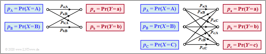 $M=2$ (left) and for $M=3$ (right). Please note: In the right graph not all transitions are labeled