Difference between revisions of "Applets:Eye Pattern and Worst-Case Error Probability"
m (Text replacement - "„" to """) |
|||
| (21 intermediate revisions by 3 users not shown) | |||
| Line 25: | Line 25: | ||
In the $p_{\rm U}$–equation mean: | In the $p_{\rm U}$–equation mean: | ||
| − | *${\rm Q}(x)$ is the [[Applets:Complementary_Gaussian_Error_Functions|Complementary Gaussian Error Function]]. The normalized eye opening can have values between $0 \le ö_{\rm norm} \le 1$ . | + | *${\rm Q}(x)$ is the [[Applets:Complementary_Gaussian_Error_Functions|"Complementary Gaussian Error Function"]]. The normalized eye opening can have values between $0 \le ö_{\rm norm} \le 1$ . |
*The maximum value $(ö_{\rm norm} = 1)$ applies to the binary Nyquist system and $ö_{\rm norm}=0$ represents a "closed eye". | *The maximum value $(ö_{\rm norm} = 1)$ applies to the binary Nyquist system and $ö_{\rm norm}=0$ represents a "closed eye". | ||
*The normalized detection noise rms value $\sigma_{\rm norm}$ depends on the adjustable parameter $10 \cdot \lg \ E_{\rm B}/N_0$ but also on the coding and the receiver concept. | *The normalized detection noise rms value $\sigma_{\rm norm}$ depends on the adjustable parameter $10 \cdot \lg \ E_{\rm B}/N_0$ but also on the coding and the receiver concept. | ||
| Line 33: | Line 33: | ||
<br> | <br> | ||
<br> | <br> | ||
| − | === | + | === System description and prerequisites=== |
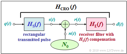
| − | + | The binary baseband transmission model outlined below applies to this applet. First, the following prerequisites apply: | |
| − | * | + | *The transmission is binary, bipolar, and redundancy-free with bit rate $R_{\rm B} = 1/T$, where $T$ is the symbol duration. |
| − | * | + | *The transmitted signal $s(t)$ is equal to $ \pm s_0$ at all times $t$ ⇒ The basic transmission pulse $g_s(t)$ is NRZ–rectangular with amplitude $s_0$ and pulse duration $T$. |
| − | * | + | *Let the received signal be $r(t) = s(t) + n(t)$, where the AWGN term $n(t)$ is characterized by the (one-sided) noise power density $N_0$. |
| − | * | + | *Let the channel frequency response be best possible (ideal) and need not be considered further: $H_{\rm K}(f) =1$. |
| − | * | + | *The receiver filter with the impulse response $h_{\rm E}(t)$ forms the detection signal $d(t) = d_{\rm S}(t)+ d_{\rm N}(t)$ from $r(t)$. |
| − | * | + | * This is evaluated by the decision with the decision threshold $E = 0$ at the equidistant times $\nu \cdot T$. |
| − | * | + | *A distinction is made between the signal component $d_{\rm S}(t)$ – originating from $s(t)$ – and the noise component $d_{\rm N}(t)$, whose cause is the AWGN noise $n(t)$. |
| − | *$d_{\rm S}(t)$ | + | *$d_{\rm S}(t)$ can be represented as a weighted sum of weighted basic detection pulses $T$, each shifted by $g_d(t) = g_s(t) \star h_{\rm E}(t)$. |
| − | * | + | *To calculate the (average) error probability, one further needs the variance $\sigma_d^2 = {\rm E}\big[d_{\rm N}(t)^2\big]$ of the detection noise component (for AWGN noise). |
| − | === | + | ===Optimal intersymbol interference-free system – matched filter receiver=== |
| − | + | The minimum error probability results for the case considered here $H_{\rm K}(f) =1$ with the matched filter receiver, i.e. when $h_{\rm E}(t)$ is equal in shape to the NRZ basic transmission pulse $g_s(t)$. The rectangular impulse response $h_{\rm E}(t)$ then has duration $T_{\rm E} = T$ and height $1/T$. | |
| − | [[File: | + | [[File:EN_Dig_T_1_4_S1_v2.png|right|frame|Binary baseband transmission system <br> <u>Note:</u> The sketch for $h_{\rm E}(t)$ applies only to the matched filter receiver ]] |
| − | * | + | *The basic detection pulse $g_d(t)$ is triangular with maximum $s_0$ at $t=0$ ; $g_d(t)=0$ for $|t| \ge T$. Due to this tight temporal constraint, there is no intersymbol interference ⇒ $d_{\rm S}(t = \nu \cdot T) = \pm s_0$ ⇒ the distance of all useful samples from the threshold $E = 0$ is always $|d_{\rm S}(t = \nu \cdot T)| = s_0$. |
| − | * | + | *The detection noise power for this constellation is: |
:$$\sigma_d^2 = N_0/2 \cdot \int_{-\infty}^{+\infty} |h_{\rm E}(t)|^2 {\rm d}t = N_0/(2T)=\sigma_{\rm MF}^2.$$ | :$$\sigma_d^2 = N_0/2 \cdot \int_{-\infty}^{+\infty} |h_{\rm E}(t)|^2 {\rm d}t = N_0/(2T)=\sigma_{\rm MF}^2.$$ | ||
| − | * | + | *For the (average) error probability, using the [[Theory_of_Stochastic_Signals/Gaussian_Distributed_Random_Variables#Exceedance_probability|"Complementary Gaussian Error Function"]] ${\rm Q}(x)$ : |
:$$p_{\rm M} = {\rm Q}\left[\sqrt{{s_0^2}/{\sigma_d^2}}\right ] = {\rm Q}\left[\sqrt{{2 \cdot s_0^2 \cdot T}/{N_0}}\right ] = {\rm Q}\left[\sqrt{2 \cdot E_{\rm B}/ N_0}\right ].$$ | :$$p_{\rm M} = {\rm Q}\left[\sqrt{{s_0^2}/{\sigma_d^2}}\right ] = {\rm Q}\left[\sqrt{{2 \cdot s_0^2 \cdot T}/{N_0}}\right ] = {\rm Q}\left[\sqrt{2 \cdot E_{\rm B}/ N_0}\right ].$$ | ||
| − | + | The applet considers this case with the settings "after gap–low-pass" as well as $T_{\rm E}/T = 1$. The output values are with regard to later constellations | |
| − | * | + | *the normalized eye opening $ö_{\rm norm} =1$ ⇒ this is the maximum possible value, |
| − | * | + | *the normalized detection noise rms value (equal to the square root of the detection noise power) $\sigma_{\rm norm} =\sqrt{1/(2 \cdot E_{\rm B}/ N_0)}$ as well as |
| − | * | + | *the worst-case error probability $p_{\rm U} = {\rm Q}\left[ö_{\rm norm}/\sigma_{\rm norm} \right ]$ ⇒ for intersymbol interference-free systems, $p_{\rm M}$ and $p_{\rm U}$ agree. |
| − | $\text{ | + | $\text{Differences in the multi-level systems}$ |
| − | * | + | *There are $M\hspace{-0.1cm}-\hspace{-0.1cm}1$ eyes and just as many thresholds ⇒ $ö_{\rm norm} =1/(M\hspace{-0.1cm}-\hspace{-0.1cm}1)$ ⇒ $M=4$: quaternary system, $M=3$: AMI code, duobinary code. |
| − | * | + | *The normalized detection noise rms value $\sigma_{\rm norm}$ is smaller by a factor of $\sqrt{5/9} \approx 0.745$ for the quaternary system than for the binary system. |
| − | * | + | *For the AMI code and the duobinary code, this improvement factor, which goes back to the smaller $E_{\rm B}/ N_0$, has the value $\sqrt{1/2} \approx 0.707$. |
<br> | <br> | ||
| − | ===Nyquist | + | ===Nyquist system with raised cosine overall frequency response=== |
| − | [[File: | + | [[File:EN_Auge_2.png|right|frame|Raised cosine overall frequency response]] |
| − | + | We assume that the overall frequency response between the Dirac-shaped source to the decision has the shape of a [[Linear_and_Time_Invariant_Systems/Some_Low-Pass_Functions_in_Systems_Theory#Raised-cosine_low-pass_filter|"raised cosine low-pass"]] ⇒ $H_{\rm S}(f)\cdot H_{\rm E}(f) = H_{\rm CRO}(f)$ . | |
| − | * | + | *The rolloff of $H_{\rm CRO}(f)$ is point symmetric about the Nyquist frequency $1/(2T)$. The larger the rolloff factor $r_{ \hspace {-0.05cm}f}$, ithe flatter the Nyquist slope. |
| − | * | + | *The basic detection pulse $g_d(t) = s_0 \cdot T \cdot {\mathcal F}^{-1}\big[H_{\rm CRO}(f)\big]$ has zeros at times $\nu \cdot T$ independent of $r_{ \hspace {-0.05cm}f}$. There are further zero crossings depending on $r_{ \hspace {-0.05cm}f}$. For the pulse holds: |
| − | :$$g_d(t) = s_0 \hspace{-0.05cm}\cdot\hspace{-0.05cm} {\rm | + | :$$g_d(t) = s_0 \hspace{-0.05cm}\cdot\hspace{-0.05cm} {\rm sinc}( t/T )\hspace{-0.05cm}\cdot\hspace{-0.05cm}\frac {\cos(\pi \cdot r_{\hspace{-0.05cm}f} \cdot t/T )}{1 - (2 \cdot |
r_{\hspace{-0.05cm}f} \cdot t/T)^2}.$$ | r_{\hspace{-0.05cm}f} \cdot t/T)^2}.$$ | ||
| − | * | + | *It follows: As with the matched filter receiver, the eye is maximally open ⇒ $ö_{\rm norm} =1$. |
| − | + | [[File:EN_Dig_T_1_4_S6.png|right|frame|Optimizing the rolloff factor]] | |
| − | [[File: | + | Let us now consider the noise power before the decision. For this holds: |
| − | |||
:$$\sigma_d^2 = N_0/2 \cdot \int_{-\infty}^{+\infty} |H_{\rm E}(f)|^2 {\rm d}f = N_0/2 \cdot \int_{-\infty}^{+\infty} \frac{|H_{\rm CRO}(f)|^2}{|H_{\rm S}(f)|^2} {\rm d}f.$$ | :$$\sigma_d^2 = N_0/2 \cdot \int_{-\infty}^{+\infty} |H_{\rm E}(f)|^2 {\rm d}f = N_0/2 \cdot \int_{-\infty}^{+\infty} \frac{|H_{\rm CRO}(f)|^2}{|H_{\rm S}(f)|^2} {\rm d}f.$$ | ||
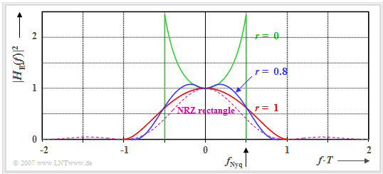
| − | + | The graph shows the power transfer function $|H_{\rm E}(f)|^2$ for three different rolloff factors | |
| − | * $r_{ \hspace {-0.05cm}f}=0$ ⇒ | + | * $r_{ \hspace {-0.05cm}f}=0$ ⇒ green curve, |
| − | * $r_{ \hspace {-0.05cm}f}=1$ ⇒ | + | * $r_{ \hspace {-0.05cm}f}=1$ ⇒ red curve, |
| − | * $r_{ \hspace {-0.05cm}f}=0.8$ ⇒ | + | * $r_{ \hspace {-0.05cm}f}=0.8$ ⇒ blue curve. |
| − | + | The areas under these curves are each a measure of the noise power $\sigma_d^2$. The rectangle with a gray background marks the smallest value $\sigma_d^2 =\sigma_{\rm MF}^2$, which also resulted with the matched filter receiver. | |
<br clear=all> | <br clear=all> | ||
| − | + | One can see from this plot: | |
| − | * | + | *The rolloff factor $r_{\hspace{-0.05cm}f} = 0$ (rectangular frequency response) leads to $\sigma_d^2 =K \cdot \sigma_{\rm MF}^2$ with $K \approx 1.5$ despite the very narrow receiver filter, since $|H_{\rm E}(f)|^2$ increases steeply as $f$ increases. The reason for this noise power increase is the $\rm sinc^2(f T)$ function in the denominator, which is required to compensate for the $|H_{\rm S}(f)|^2$–decay. <br> |
| − | * | + | * Since the area under the red curve is smaller than that under the green curve, $r_{\hspace{-0.05cm}f} = 1$ leads to a smaller noise power despite a spectrum twice as wide: $K \approx 1.23$. For $r_{\hspace{-0.05cm}f} \approx 0.8$, a slightly better value results. For this, the best possible compromise between bandwidth and excess noise is achieved. |
| − | * | + | *The normalized detection noise rms value is thus for the rolloff factor $r_{ \hspace {-0.05cm}f}$: $\sigma_{\rm norm} =\sqrt{K(r_f)/(2 \cdot E_{\rm B}/ N_0)}$. <br> |
| − | * | + | *Again, the worst-case error probability $p_{\rm U} = {\rm Q}\left[ö_{\rm norm}/\sigma_{\rm norm} \right ]$ coincides exactly with the mean error probability $p_{\rm M}$. |
| − | $\text{ | + | $\text{Differences in the multi-level systems}$ |
| − | + | All remarks in section $2.2$ apply in the same way to the "Nyquist system with raised cosine total frequency response". | |
| − | === | + | ===Intersymbol interference system with Gaussian receiver filter=== |
| − | [[File: | + | [[File:EN_Auge_4_neu.png|right|frame|System with Gaussian receiver filter]] |
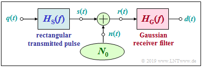
| − | + | We start from the block diagram sketched on the right. Further it shall be valid: | |
| − | * | + | *Rectangular NRZ basic transmission pulse $g_s(t)$ with height $s_0$ and duration $T$: |
| − | :$$H_{\rm S}(f) = {\rm | + | :$$H_{\rm S}(f) = {\rm sinc}(f T).$$ |
| − | * | + | *Gaussian receiver filter with cutoff frequency $f_{\rm G}$: |
:$$H_{\rm E}(f) = H_{\rm G}(f) = {\rm e}^{- \pi \hspace{0.05cm}\cdot \hspace{0.03cm} f^2/(2\hspace{0.05cm}\cdot \hspace{0.03cm}f_{\rm G})^2 } \hspace{0.2cm} \bullet\!\!-\!\!\!-\!\!\!-\!\!\circ | :$$H_{\rm E}(f) = H_{\rm G}(f) = {\rm e}^{- \pi \hspace{0.05cm}\cdot \hspace{0.03cm} f^2/(2\hspace{0.05cm}\cdot \hspace{0.03cm}f_{\rm G})^2 } \hspace{0.2cm} \bullet\!\!-\!\!\!-\!\!\!-\!\!\circ | ||
\hspace{0.2cm}h_{\rm E}(t) = h_{\rm G}(t) = {\rm e}^{- \pi \cdot (2\hspace{0.05cm}\cdot \hspace{0.03cm} | \hspace{0.2cm}h_{\rm E}(t) = h_{\rm G}(t) = {\rm e}^{- \pi \cdot (2\hspace{0.05cm}\cdot \hspace{0.03cm} | ||
| Line 124: | Line 123: | ||
\hspace{0.05cm}.$$ | \hspace{0.05cm}.$$ | ||
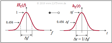
| − | + | Based on the assumptions made here, the following applies to the basic detection pulse: | |
| − | [[File:Auge_5_neu.png|right|frame| | + | [[File:Auge_5_neu.png|right|frame|Frequency response and impulse response of the receiver filter]] |
:$$g_d(t) = s_0 \cdot T \cdot \big [h_{\rm S}(t) \star h_{\rm G}(t)\big ] = 2 f_{\rm G} \cdot s_0 \cdot \int_{t-T/2}^{t+T/2} | :$$g_d(t) = s_0 \cdot T \cdot \big [h_{\rm S}(t) \star h_{\rm G}(t)\big ] = 2 f_{\rm G} \cdot s_0 \cdot \int_{t-T/2}^{t+T/2} | ||
{\rm e}^{- \pi \hspace{0.05cm}\cdot\hspace{0.05cm} (2 \hspace{0.05cm}\cdot\hspace{0.02cm} | {\rm e}^{- \pi \hspace{0.05cm}\cdot\hspace{0.05cm} (2 \hspace{0.05cm}\cdot\hspace{0.02cm} | ||
f_{\rm G}\hspace{0.05cm}\cdot\hspace{0.02cm} \tau )^2} \,{\rm d} \tau \hspace{0.05cm}.$$ | f_{\rm G}\hspace{0.05cm}\cdot\hspace{0.02cm} \tau )^2} \,{\rm d} \tau \hspace{0.05cm}.$$ | ||
| − | + | The integration leads to the result: | |
:$$g_d(t) = s_0 \cdot \big [ {\rm Q} \left ( 2 \cdot \sqrt {2 \pi} | :$$g_d(t) = s_0 \cdot \big [ {\rm Q} \left ( 2 \cdot \sqrt {2 \pi} | ||
| Line 138: | Line 137: | ||
)\right ) \big ],$$ | )\right ) \big ],$$ | ||
| − | + | using the complementary Gaussian error function | |
:$${\rm Q} (x) = \frac{\rm 1}{\sqrt{\rm 2\pi}}\int_{\it | :$${\rm Q} (x) = \frac{\rm 1}{\sqrt{\rm 2\pi}}\int_{\it | ||
| Line 144: | Line 143: | ||
\hspace{0.05cm}.$$ | \hspace{0.05cm}.$$ | ||
| − | + | The module [[Applets:Komplementäre_Gaußsche_Fehlerfunktionen|"Complementary Gaussian Error Functions"]] provides the numerical values of ${\rm Q} (x)$.<br> | |
| − | * | + | *This basic detection pulse causes [[Digital_Signal_Transmission/Causes_and_Effects_of_Intersymbol_Interference#Definition_of_the_term_.22Intersymbol_Interference.22|"intersymbol interference"]]. |
| − | * | + | *This is understood to mean that the symbol decision is influenced by the spurs of neighboring pulses. While in intersymbol interference free transmission systems each symbol is falsified with the same probability – namely the mean error probability $p_{\rm M}$ – there are favorable symbol combinations with the falsification probability ${\rm Pr}(v_{\nu} \ne q_{\nu}) < p_{\rm M}$. |
| − | * | + | *In contrast, other symbol combinations increase the falsification probability significantly. |
| − | [[File:Auge_6.png|right|frame| | + | [[File:Auge_6.png|right|frame|Binary eye $($Gaussian low-pass, $f_{\rm G}/R_{\rm B} = 0.35)$.]] |
| − | + | The intersymbol interferences can be captured and analyzed very easily by the so-called '''eye diagram'''. These are the focus of this applet. All important information can be found [[Digital_Signal_Transmission/Error_Probability_with_Intersymbol_Interference#Definition_and_statements_of_the_eye_diagram|"here"]]. | |
| − | * | + | *The eye diagram is created by drawing all sections of the detection useful signal $d_{\rm S}(t)$ of length $2T$ on top of each other. You can visualize the formation in the program with "single step". |
| − | * | + | * A measure for the strength of the intersymbol interference is the ''vertical eye opening''. For the symmetric binary case, with $g_\nu = g_d(\pm \nu \cdot T)$ and appropriate normalization: |
:$$ ö_{\rm norm} = g_0 -2 \cdot (|g_1| + |g_2| + \text{...}).$$ | :$$ ö_{\rm norm} = g_0 -2 \cdot (|g_1| + |g_2| + \text{...}).$$ | ||
| − | * | + | * With larger cutoff frequency, the pulses interfere less and $ ö_{\rm norm}$ increases continuously. At the same time, with larger $f_{\rm G}/R_{\rm B}$, the (normalized) detection noise rms value also becomes larger: |
:$$ \sigma_{\rm norm} = \sqrt{\frac{f_{\rm G}/R_{\rm B}}{\sqrt{2} \cdot E_{\rm B}/N_{\rm 0}}}.$$ | :$$ \sigma_{\rm norm} = \sqrt{\frac{f_{\rm G}/R_{\rm B}}{\sqrt{2} \cdot E_{\rm B}/N_{\rm 0}}}.$$ | ||
| − | * | + | *The worst-case error probability $p_{\rm U} = {\rm Q}\left[ö_{\rm norm}/\sigma_{\rm norm} \right ]$ ⇒ "Worst Case" is usually significantly higher than the mean error probability $p_{\rm M}$. |
| + | |||
| + | $\text{Differences in the redundancy-free quaternary system}$ | ||
| + | *For $M=4$, other basic pulse values result. <br>''Example'': With $M=4, \ f_{\rm G}/R_{\rm B}=0.4$ basic pulse values $g_0 = 0.955, \ g_1 = 0.022$ are identical with $M=2, \ f_{\rm G}/R_{\rm B}=0.8$. | ||
| + | * There are now three eye openings and just as many thresholds. The equation for the normalized eye opening is now: $ ö_{\rm norm} = g_0/3 -2 \cdot (|g_1| + |g_2| + \text{...}).$ | ||
| + | *The normalized detection noise rms $\sigma_{\rm norm}$ is again a factor of $\sqrt{5/9} \approx 0.745$ smaller for the quaternary system than for the binary system. | ||
| − | |||
| − | |||
| − | |||
| − | |||
| + | ===Pseudo-ternary codes=== | ||
| − | = | + | In symbolwise coding, each incoming source symbol $q_\nu$ generates an encoder symbol $c_\nu$ that depends not only on the current input symbol $q_\nu$ but also on the $N_{\rm C}$ preceding symbols $q_{\nu-1}$, ... , $q_{\nu-N_{\rm C}} $. $N_{\rm C}$ is referred to as the ''order'' of the code. It is typical for a symbolwise coding that |
| + | [[File:EN_Dig_T_2_4_S1_v26.png|right|frame|Block diagram and equivalent circuit of a pseudo-ternary encoder|class=fit]] | ||
| − | + | *the symbol duration $T$ of the encoded signal (and of the transmitted signal) coincides with the bit duration $T_{\rm B}$ of the binary source signal, and | |
| − | * | + | *coding and decoding do not lead to major time delays, which are unavoidable when block codes are used.<br><br> |
| − | * | ||
| − | |||
| − | + | Special importance has ''pseudo-ternary codes'' ⇒ level number $M = 3$, which can be described by the block diagram according to the left graphic. In the right graphic an equivalent circuit is given, which is very suitable for an analysis of these codes. More details can be found in the [[Digital_Signal_Transmission/Symbolwise_Coding_with_Pseudo-Ternary_Codes|"$\rm LNTwww$ theory section"]]. Conclusion: | |
| − | * | + | *Recoding from binary $(M_q = 2)$ to ternary $(M = M_c = 3)$: |
:$$q_\nu \in \{-1, +1\},\hspace{0.5cm} c_\nu \in \{-1, \ 0, +1\}\hspace{0.05cm}.$$ | :$$q_\nu \in \{-1, +1\},\hspace{0.5cm} c_\nu \in \{-1, \ 0, +1\}\hspace{0.05cm}.$$ | ||
| − | * | + | *The relative code redundancy is the same for all pseudo-ternary codes: |
:$$ r_c = 1 -1/\log_2\hspace{0.05cm}(3) \approx 36.9 \%\hspace{0.05cm}.$$ | :$$ r_c = 1 -1/\log_2\hspace{0.05cm}(3) \approx 36.9 \%\hspace{0.05cm}.$$ | ||
| − | + | Based on the code parameter $K_{\rm C}$, different first-order pseudo-ternary codes $(N_{\rm C} = 1)$ are characterized. | |
| − | [[File:Auge_16.png|right|frame| | + | [[File:Auge_16.png|right|frame|Signals in AMI coding|class=fit]] |
| − | $\Rightarrow \ \ K_{\rm C} = 1\text{: AMI | + | $\Rightarrow \ \ K_{\rm C} = 1\text{: AMI code}$ (from: ''Alternate Mark Inversion'') |
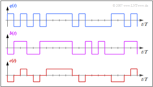
| − | + | The graph shows the binary source signal $q(t)$ at the top. Below are shown: | |
| − | * | + | * the likewise binary signal $b(t)$ after the pre-encoder, and |
| − | * | + | * the encoded signal $c(t) = s(t)$ of the AMI code. |
| − | + | One can see the simple AMI coding principle: | |
| − | * | + | *Each binary value "–1" of $q(t)$ ⇒ symbol $\rm L$ is encoded by the ternary amplitude coefficient $a_\nu = 0$. <br> |
| − | * | + | *The binary value "+1" of $q(t)$ ⇒ symbol $\rm H$ is alternately represented by $a_\nu = +1$ and $a_\nu = -1$. <br><br> |
| − | + | This ensures that there are no long "+1"– or "–1" sequences in the AMI-encoded signal, which would be problematic for an DC signal-free channel. | |
<br> | <br> | ||
| − | [[File: | + | [[File:EN_Auge_16a.png|left|frame| |class=fit]] |
| − | + | The eye diagram is shown on the left. | |
| − | ::* | + | ::* There are two eye openings and two thresholds. |
| − | ::* | + | ::* The normalized eye opening is $ö_{\rm norm}= 1/2 \cdot (g_0 -3 \cdot g_1)$, where $g_0 = g_d(t=0)$ denotes the main value of the basic detection pulse and $g_1 = g_d(t=\pm T)$ denotes the relevant precursors and postcursors that vertically limit the eye. |
| − | ::* | + | ::* The normalized eye opening is thus significantly smaller than for the comparable binary system ⇒ $ö_{\rm norm}= g_0 -2 \cdot g_1$. |
| − | ::* | + | ::* The normalized noise rms $\sigma_{\rm norm}$ is smaller than for the comparable binary system by a factor of $\sqrt{1/2} \approx 0.707$. |
<br clear=all> | <br clear=all> | ||
| − | [[File:Auge_17.png|right|frame| | + | [[File:Auge_17.png|right|frame|Signals in duobinary coding|class=fit]] |
| − | $\Rightarrow \ \ K_{\rm C} = -1\text{: | + | $\Rightarrow \ \ K_{\rm C} = -1\text{: duobinary code}$ |
| − | + | From the right graph with the signal curves one recognizes: | |
| − | * | + | *Here, any number of symbols of the same polarity ("+1" or "–1") can directly follow each other ⇒ the duobinary code is not free of DC signals. |
| − | * | + | *In contrast, the alternating sequence " ... , +1, –1, +1, –1, +1, ... " does not occur, which is particularly disturbing with regard to intersymbol interference. |
| − | * | + | * Also the duobinary encoded sequence consists to 50% of zeros. The enhancement factor due to the smaller $E_{\rm B}/ N_0$ is equal to $\sqrt{1/2} \approx 0.707$, as in the AMI code. |
| − | [[File: | + | [[File:EN_Auge_17a.png|left|frame| |class=fit]] |
<br> | <br> | ||
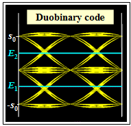
| − | + | The eye diagram is shown on the left. | |
| − | ::* | + | ::* There are again two "eyes" and two thresholds. |
| − | ::* | + | ::* The eye opening is $ö_{\rm norm}= 1/2 \cdot (g_0 - g_1)$. |
| − | *$ö_{\rm norm}$ | + | *$ö_{\rm norm}$ is thus larger than in the AMI code and also as in the comparable binary system. |
| − | * | + | *A disadvantage compared to the AMI code, however, is that it is not DC signal-free. |
| Line 331: | Line 331: | ||
==Applet Manual== | ==Applet Manual== | ||
<br> | <br> | ||
| − | [[File:Anleitung_Auge.png|right|600px]] | + | [[File:Anleitung_Auge.png|right|600px|frame|Screenshot of the German version]] |
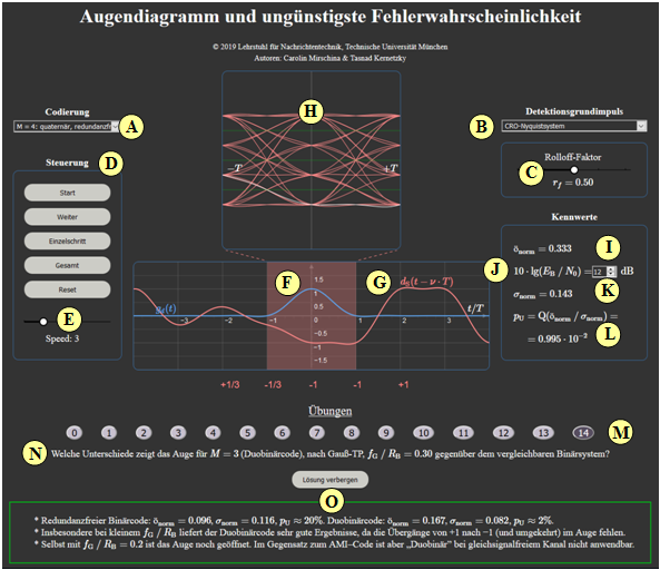
| − | '''(A)''' | + | '''(A)''' Selection: Encoding <br> (binary, quaternary, AMI code, duobinary code) |
| − | '''(B)''' | + | '''(B)''' Selection: Basic detection pulse<br> (according to Gauss–TP, CRO–Nyquist, according to gap–TP} |
| − | '''(C)''' | + | '''(C)''' Parameter input for '''(B)'''<br> (cutoff frequency, rolloff factor, rectangular duration) |
| − | '''(D)''' | + | '''(D)''' Control of the eye diagram display<br> (start, pause/continue, single step, total, reset) |
| − | '''(E)''' | + | '''(E)''' Speed of the eye diagram display |
| − | '''(F)''' | + | '''(F)''' Display: basic detection pulse $g_d(t)$ |
| − | '''(G)''' | + | '''(G)''' Display: detection useful signal $d_{\rm S}(t - \nu \cdot T)$ |
| − | '''(H)''' | + | '''(H)''' Display: eye diagram in the range $\pm T$ |
| − | '''( I )''' | + | '''( I )''' Numerical output: $ö_{\rm norm}$ (normalized eye opening) |
| − | '''(J)''' | + | '''(J)''' Parameter input $10 \cdot \lg \ E_{\rm B}/N_0$ for '''(K)''' |
| − | '''(K)''' | + | '''(K)''' Numerical output: $\sigma_{\rm norm}$ (normalized noise rms) |
| − | '''(L)''' | + | '''(L)''' Numerical output: $p_{\rm U}$ (worst-case error probability) |
| − | '''(M)''' | + | '''(M)''' Range for experimental performance: task selection |
| − | '''(N)''' | + | '''(N)''' Range for experimental performance: task description |
| − | '''(O)''' | + | '''(O)''' Range for experimental performance: Show sample solution |
<br clear=all> | <br clear=all> | ||
==About the Authors== | ==About the Authors== | ||
This interactive calculation tool was designed and implemented at the [https://www.ei.tum.de/en/lnt/home/ Institute for Communications Engineering] at the [https://www.tum.de/en Technical University of Munich]. | This interactive calculation tool was designed and implemented at the [https://www.ei.tum.de/en/lnt/home/ Institute for Communications Engineering] at the [https://www.tum.de/en Technical University of Munich]. | ||
| − | *The first version was created in 2008 by [[ | + | *The first version was created in 2008 by [[Biographies_and_Bibliographies/Students_involved_in_LNTwww#Thomas_Gro.C3.9Fer_.28Diplomarbeit_LB_2006.2C_danach_freie_Mitarbeit_bis_2010.29|Thomas Großer]] as part of his diploma thesis with “FlashMX – Actionscript” (Supervisor: [[Biographies_and_Bibliographies/LNTwww_members_from_LNT#Prof._Dr.-Ing._habil._G.C3.BCnter_S.C3.B6der_.28am_LNT_seit_1974.29|Günter Söder]]). |
| − | *Last revision and English version 2020/2021 by [[ | + | *Last revision and English version 2020/2021 by [[Biographies_and_Bibliographies/Students_involved_in_LNTwww#Carolin_Mirschina_.28Ingenieurspraxis_Math_2019.2C_danach_Werkstudentin.29|Carolin Mirschina]] in the context of a working student activity. |
Latest revision as of 16:06, 17 January 2024
Open Applet in new Tab Deutsche Version Öffnen
Contents
Applet Description
The applet illustrates the eye pattern for different encodings
- binary (redundancy-free),
- quaternary (redundancy-free),
- pseudo–ternary: (AMI and duobinary)
and for various reception concepts
- Matched Filter receiver,
- CRO Nyquist system,
- Gaussian low-pass filter.
The last reception concept leads to intersymbol interference, that is: Neighboring symbols interfere with each other in symbol decision.
Such intersymbol interferences and their influence on the error probability can be captured and quantified very easily by the "eye pattern". But also for the other two (without intersymbol interference) systems important insights can be gained from the graphs.
Furthermore, the most unfavorable ("worst case") error probability
- $$p_{\rm U} = {\rm Q}\left[ö_{\rm norm}/\sigma_{\rm norm} \right ]$$
is output, which for binary Nyquist systems is identical to the mean error probability $p_{\rm M}$ and represents a suitable upper bound for the other system variants: $p_{\rm U} \ge p_{\rm M}$.
In the $p_{\rm U}$–equation mean:
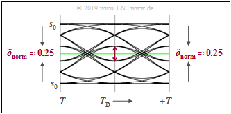
- ${\rm Q}(x)$ is the "Complementary Gaussian Error Function". The normalized eye opening can have values between $0 \le ö_{\rm norm} \le 1$ .
- The maximum value $(ö_{\rm norm} = 1)$ applies to the binary Nyquist system and $ö_{\rm norm}=0$ represents a "closed eye".
- The normalized detection noise rms value $\sigma_{\rm norm}$ depends on the adjustable parameter $10 \cdot \lg \ E_{\rm B}/N_0$ but also on the coding and the receiver concept.
Theoretical Background
System description and prerequisites
The binary baseband transmission model outlined below applies to this applet. First, the following prerequisites apply:
- The transmission is binary, bipolar, and redundancy-free with bit rate $R_{\rm B} = 1/T$, where $T$ is the symbol duration.
- The transmitted signal $s(t)$ is equal to $ \pm s_0$ at all times $t$ ⇒ The basic transmission pulse $g_s(t)$ is NRZ–rectangular with amplitude $s_0$ and pulse duration $T$.
- Let the received signal be $r(t) = s(t) + n(t)$, where the AWGN term $n(t)$ is characterized by the (one-sided) noise power density $N_0$.
- Let the channel frequency response be best possible (ideal) and need not be considered further: $H_{\rm K}(f) =1$.
- The receiver filter with the impulse response $h_{\rm E}(t)$ forms the detection signal $d(t) = d_{\rm S}(t)+ d_{\rm N}(t)$ from $r(t)$.
- This is evaluated by the decision with the decision threshold $E = 0$ at the equidistant times $\nu \cdot T$.
- A distinction is made between the signal component $d_{\rm S}(t)$ – originating from $s(t)$ – and the noise component $d_{\rm N}(t)$, whose cause is the AWGN noise $n(t)$.
- $d_{\rm S}(t)$ can be represented as a weighted sum of weighted basic detection pulses $T$, each shifted by $g_d(t) = g_s(t) \star h_{\rm E}(t)$.
- To calculate the (average) error probability, one further needs the variance $\sigma_d^2 = {\rm E}\big[d_{\rm N}(t)^2\big]$ of the detection noise component (for AWGN noise).
Optimal intersymbol interference-free system – matched filter receiver
The minimum error probability results for the case considered here $H_{\rm K}(f) =1$ with the matched filter receiver, i.e. when $h_{\rm E}(t)$ is equal in shape to the NRZ basic transmission pulse $g_s(t)$. The rectangular impulse response $h_{\rm E}(t)$ then has duration $T_{\rm E} = T$ and height $1/T$.
- The basic detection pulse $g_d(t)$ is triangular with maximum $s_0$ at $t=0$ ; $g_d(t)=0$ for $|t| \ge T$. Due to this tight temporal constraint, there is no intersymbol interference ⇒ $d_{\rm S}(t = \nu \cdot T) = \pm s_0$ ⇒ the distance of all useful samples from the threshold $E = 0$ is always $|d_{\rm S}(t = \nu \cdot T)| = s_0$.
- The detection noise power for this constellation is:
- $$\sigma_d^2 = N_0/2 \cdot \int_{-\infty}^{+\infty} |h_{\rm E}(t)|^2 {\rm d}t = N_0/(2T)=\sigma_{\rm MF}^2.$$
- For the (average) error probability, using the "Complementary Gaussian Error Function" ${\rm Q}(x)$ :
- $$p_{\rm M} = {\rm Q}\left[\sqrt{{s_0^2}/{\sigma_d^2}}\right ] = {\rm Q}\left[\sqrt{{2 \cdot s_0^2 \cdot T}/{N_0}}\right ] = {\rm Q}\left[\sqrt{2 \cdot E_{\rm B}/ N_0}\right ].$$
The applet considers this case with the settings "after gap–low-pass" as well as $T_{\rm E}/T = 1$. The output values are with regard to later constellations
- the normalized eye opening $ö_{\rm norm} =1$ ⇒ this is the maximum possible value,
- the normalized detection noise rms value (equal to the square root of the detection noise power) $\sigma_{\rm norm} =\sqrt{1/(2 \cdot E_{\rm B}/ N_0)}$ as well as
- the worst-case error probability $p_{\rm U} = {\rm Q}\left[ö_{\rm norm}/\sigma_{\rm norm} \right ]$ ⇒ for intersymbol interference-free systems, $p_{\rm M}$ and $p_{\rm U}$ agree.
$\text{Differences in the multi-level systems}$
- There are $M\hspace{-0.1cm}-\hspace{-0.1cm}1$ eyes and just as many thresholds ⇒ $ö_{\rm norm} =1/(M\hspace{-0.1cm}-\hspace{-0.1cm}1)$ ⇒ $M=4$: quaternary system, $M=3$: AMI code, duobinary code.
- The normalized detection noise rms value $\sigma_{\rm norm}$ is smaller by a factor of $\sqrt{5/9} \approx 0.745$ for the quaternary system than for the binary system.
- For the AMI code and the duobinary code, this improvement factor, which goes back to the smaller $E_{\rm B}/ N_0$, has the value $\sqrt{1/2} \approx 0.707$.
Nyquist system with raised cosine overall frequency response
We assume that the overall frequency response between the Dirac-shaped source to the decision has the shape of a "raised cosine low-pass" ⇒ $H_{\rm S}(f)\cdot H_{\rm E}(f) = H_{\rm CRO}(f)$ .
- The rolloff of $H_{\rm CRO}(f)$ is point symmetric about the Nyquist frequency $1/(2T)$. The larger the rolloff factor $r_{ \hspace {-0.05cm}f}$, ithe flatter the Nyquist slope.
- The basic detection pulse $g_d(t) = s_0 \cdot T \cdot {\mathcal F}^{-1}\big[H_{\rm CRO}(f)\big]$ has zeros at times $\nu \cdot T$ independent of $r_{ \hspace {-0.05cm}f}$. There are further zero crossings depending on $r_{ \hspace {-0.05cm}f}$. For the pulse holds:
- $$g_d(t) = s_0 \hspace{-0.05cm}\cdot\hspace{-0.05cm} {\rm sinc}( t/T )\hspace{-0.05cm}\cdot\hspace{-0.05cm}\frac {\cos(\pi \cdot r_{\hspace{-0.05cm}f} \cdot t/T )}{1 - (2 \cdot r_{\hspace{-0.05cm}f} \cdot t/T)^2}.$$
- It follows: As with the matched filter receiver, the eye is maximally open ⇒ $ö_{\rm norm} =1$.
Let us now consider the noise power before the decision. For this holds:
- $$\sigma_d^2 = N_0/2 \cdot \int_{-\infty}^{+\infty} |H_{\rm E}(f)|^2 {\rm d}f = N_0/2 \cdot \int_{-\infty}^{+\infty} \frac{|H_{\rm CRO}(f)|^2}{|H_{\rm S}(f)|^2} {\rm d}f.$$
The graph shows the power transfer function $|H_{\rm E}(f)|^2$ for three different rolloff factors
- $r_{ \hspace {-0.05cm}f}=0$ ⇒ green curve,
- $r_{ \hspace {-0.05cm}f}=1$ ⇒ red curve,
- $r_{ \hspace {-0.05cm}f}=0.8$ ⇒ blue curve.
The areas under these curves are each a measure of the noise power $\sigma_d^2$. The rectangle with a gray background marks the smallest value $\sigma_d^2 =\sigma_{\rm MF}^2$, which also resulted with the matched filter receiver.
One can see from this plot:
- The rolloff factor $r_{\hspace{-0.05cm}f} = 0$ (rectangular frequency response) leads to $\sigma_d^2 =K \cdot \sigma_{\rm MF}^2$ with $K \approx 1.5$ despite the very narrow receiver filter, since $|H_{\rm E}(f)|^2$ increases steeply as $f$ increases. The reason for this noise power increase is the $\rm sinc^2(f T)$ function in the denominator, which is required to compensate for the $|H_{\rm S}(f)|^2$–decay.
- Since the area under the red curve is smaller than that under the green curve, $r_{\hspace{-0.05cm}f} = 1$ leads to a smaller noise power despite a spectrum twice as wide: $K \approx 1.23$. For $r_{\hspace{-0.05cm}f} \approx 0.8$, a slightly better value results. For this, the best possible compromise between bandwidth and excess noise is achieved.
- The normalized detection noise rms value is thus for the rolloff factor $r_{ \hspace {-0.05cm}f}$: $\sigma_{\rm norm} =\sqrt{K(r_f)/(2 \cdot E_{\rm B}/ N_0)}$.
- Again, the worst-case error probability $p_{\rm U} = {\rm Q}\left[ö_{\rm norm}/\sigma_{\rm norm} \right ]$ coincides exactly with the mean error probability $p_{\rm M}$.
$\text{Differences in the multi-level systems}$
All remarks in section $2.2$ apply in the same way to the "Nyquist system with raised cosine total frequency response".
Intersymbol interference system with Gaussian receiver filter
We start from the block diagram sketched on the right. Further it shall be valid:
- Rectangular NRZ basic transmission pulse $g_s(t)$ with height $s_0$ and duration $T$:
- $$H_{\rm S}(f) = {\rm sinc}(f T).$$
- Gaussian receiver filter with cutoff frequency $f_{\rm G}$:
- $$H_{\rm E}(f) = H_{\rm G}(f) = {\rm e}^{- \pi \hspace{0.05cm}\cdot \hspace{0.03cm} f^2/(2\hspace{0.05cm}\cdot \hspace{0.03cm}f_{\rm G})^2 } \hspace{0.2cm} \bullet\!\!-\!\!\!-\!\!\!-\!\!\circ \hspace{0.2cm}h_{\rm E}(t) = h_{\rm G}(t) = {\rm e}^{- \pi \cdot (2\hspace{0.05cm}\cdot \hspace{0.03cm} f_{\rm G}\hspace{0.05cm}\cdot \hspace{0.02cm} t)^2} \hspace{0.05cm}.$$
Based on the assumptions made here, the following applies to the basic detection pulse:
- $$g_d(t) = s_0 \cdot T \cdot \big [h_{\rm S}(t) \star h_{\rm G}(t)\big ] = 2 f_{\rm G} \cdot s_0 \cdot \int_{t-T/2}^{t+T/2} {\rm e}^{- \pi \hspace{0.05cm}\cdot\hspace{0.05cm} (2 \hspace{0.05cm}\cdot\hspace{0.02cm} f_{\rm G}\hspace{0.05cm}\cdot\hspace{0.02cm} \tau )^2} \,{\rm d} \tau \hspace{0.05cm}.$$
The integration leads to the result:
- $$g_d(t) = s_0 \cdot \big [ {\rm Q} \left ( 2 \cdot \sqrt {2 \pi} \cdot f_{\rm G}\cdot ( t - {T}/{2})\right )- {\rm Q} \left ( 2 \cdot \sqrt {2 \pi} \cdot f_{\rm G}\cdot ( t + {T}/{2} )\right ) \big ],$$
using the complementary Gaussian error function
- $${\rm Q} (x) = \frac{\rm 1}{\sqrt{\rm 2\pi}}\int_{\it x}^{+\infty}\rm e^{\it -u^{\rm 2}/\rm 2}\,d {\it u} \hspace{0.05cm}.$$
The module "Complementary Gaussian Error Functions" provides the numerical values of ${\rm Q} (x)$.
- This basic detection pulse causes "intersymbol interference".
- This is understood to mean that the symbol decision is influenced by the spurs of neighboring pulses. While in intersymbol interference free transmission systems each symbol is falsified with the same probability – namely the mean error probability $p_{\rm M}$ – there are favorable symbol combinations with the falsification probability ${\rm Pr}(v_{\nu} \ne q_{\nu}) < p_{\rm M}$.
- In contrast, other symbol combinations increase the falsification probability significantly.
The intersymbol interferences can be captured and analyzed very easily by the so-called eye diagram. These are the focus of this applet. All important information can be found "here".
- The eye diagram is created by drawing all sections of the detection useful signal $d_{\rm S}(t)$ of length $2T$ on top of each other. You can visualize the formation in the program with "single step".
- A measure for the strength of the intersymbol interference is the vertical eye opening. For the symmetric binary case, with $g_\nu = g_d(\pm \nu \cdot T)$ and appropriate normalization:
- $$ ö_{\rm norm} = g_0 -2 \cdot (|g_1| + |g_2| + \text{...}).$$
- With larger cutoff frequency, the pulses interfere less and $ ö_{\rm norm}$ increases continuously. At the same time, with larger $f_{\rm G}/R_{\rm B}$, the (normalized) detection noise rms value also becomes larger:
- $$ \sigma_{\rm norm} = \sqrt{\frac{f_{\rm G}/R_{\rm B}}{\sqrt{2} \cdot E_{\rm B}/N_{\rm 0}}}.$$
- The worst-case error probability $p_{\rm U} = {\rm Q}\left[ö_{\rm norm}/\sigma_{\rm norm} \right ]$ ⇒ "Worst Case" is usually significantly higher than the mean error probability $p_{\rm M}$.
$\text{Differences in the redundancy-free quaternary system}$
- For $M=4$, other basic pulse values result.
Example: With $M=4, \ f_{\rm G}/R_{\rm B}=0.4$ basic pulse values $g_0 = 0.955, \ g_1 = 0.022$ are identical with $M=2, \ f_{\rm G}/R_{\rm B}=0.8$. - There are now three eye openings and just as many thresholds. The equation for the normalized eye opening is now: $ ö_{\rm norm} = g_0/3 -2 \cdot (|g_1| + |g_2| + \text{...}).$
- The normalized detection noise rms $\sigma_{\rm norm}$ is again a factor of $\sqrt{5/9} \approx 0.745$ smaller for the quaternary system than for the binary system.
Pseudo-ternary codes
In symbolwise coding, each incoming source symbol $q_\nu$ generates an encoder symbol $c_\nu$ that depends not only on the current input symbol $q_\nu$ but also on the $N_{\rm C}$ preceding symbols $q_{\nu-1}$, ... , $q_{\nu-N_{\rm C}} $. $N_{\rm C}$ is referred to as the order of the code. It is typical for a symbolwise coding that
- the symbol duration $T$ of the encoded signal (and of the transmitted signal) coincides with the bit duration $T_{\rm B}$ of the binary source signal, and
- coding and decoding do not lead to major time delays, which are unavoidable when block codes are used.
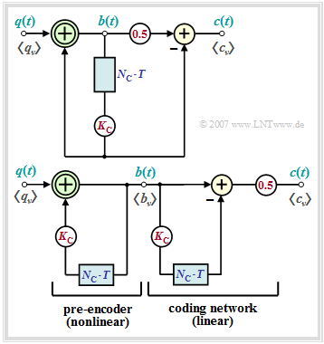
Special importance has pseudo-ternary codes ⇒ level number $M = 3$, which can be described by the block diagram according to the left graphic. In the right graphic an equivalent circuit is given, which is very suitable for an analysis of these codes. More details can be found in the "$\rm LNTwww$ theory section". Conclusion:
- Recoding from binary $(M_q = 2)$ to ternary $(M = M_c = 3)$:
- $$q_\nu \in \{-1, +1\},\hspace{0.5cm} c_\nu \in \{-1, \ 0, +1\}\hspace{0.05cm}.$$
- The relative code redundancy is the same for all pseudo-ternary codes:
- $$ r_c = 1 -1/\log_2\hspace{0.05cm}(3) \approx 36.9 \%\hspace{0.05cm}.$$
Based on the code parameter $K_{\rm C}$, different first-order pseudo-ternary codes $(N_{\rm C} = 1)$ are characterized.
$\Rightarrow \ \ K_{\rm C} = 1\text{: AMI code}$ (from: Alternate Mark Inversion)
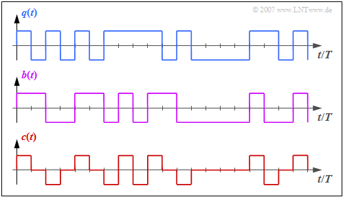
The graph shows the binary source signal $q(t)$ at the top. Below are shown:
- the likewise binary signal $b(t)$ after the pre-encoder, and
- the encoded signal $c(t) = s(t)$ of the AMI code.
One can see the simple AMI coding principle:
- Each binary value "–1" of $q(t)$ ⇒ symbol $\rm L$ is encoded by the ternary amplitude coefficient $a_\nu = 0$.
- The binary value "+1" of $q(t)$ ⇒ symbol $\rm H$ is alternately represented by $a_\nu = +1$ and $a_\nu = -1$.
This ensures that there are no long "+1"– or "–1" sequences in the AMI-encoded signal, which would be problematic for an DC signal-free channel.
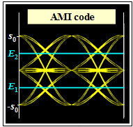
The eye diagram is shown on the left.
- There are two eye openings and two thresholds.
- The normalized eye opening is $ö_{\rm norm}= 1/2 \cdot (g_0 -3 \cdot g_1)$, where $g_0 = g_d(t=0)$ denotes the main value of the basic detection pulse and $g_1 = g_d(t=\pm T)$ denotes the relevant precursors and postcursors that vertically limit the eye.
- The normalized eye opening is thus significantly smaller than for the comparable binary system ⇒ $ö_{\rm norm}= g_0 -2 \cdot g_1$.
- The normalized noise rms $\sigma_{\rm norm}$ is smaller than for the comparable binary system by a factor of $\sqrt{1/2} \approx 0.707$.
$\Rightarrow \ \ K_{\rm C} = -1\text{: duobinary code}$
From the right graph with the signal curves one recognizes:
- Here, any number of symbols of the same polarity ("+1" or "–1") can directly follow each other ⇒ the duobinary code is not free of DC signals.
- In contrast, the alternating sequence " ... , +1, –1, +1, –1, +1, ... " does not occur, which is particularly disturbing with regard to intersymbol interference.
- Also the duobinary encoded sequence consists to 50% of zeros. The enhancement factor due to the smaller $E_{\rm B}/ N_0$ is equal to $\sqrt{1/2} \approx 0.707$, as in the AMI code.
The eye diagram is shown on the left.
- There are again two "eyes" and two thresholds.
- The eye opening is $ö_{\rm norm}= 1/2 \cdot (g_0 - g_1)$.
- $ö_{\rm norm}$ is thus larger than in the AMI code and also as in the comparable binary system.
- A disadvantage compared to the AMI code, however, is that it is not DC signal-free.
Exercises
- First select the number $(1,\ 2, \text{...})$ of the exercise. The number $0$ corresponds to a "Reset": Same setting as at program start.
- A task description is displayed. The parameter values are adjusted. Solution after pressing "Show solution".
(1) Explain the occurrence of the eye pattern for $M=2 \text{, Gaussian low-pass, }f_{\rm G}/R_{\rm B} = 0.48$. For this, select "step–by–step".
- The eye pattern is obtained by dividing the "useful" signal $d_{\rm S}(t)$ (without noise) into pieces of duration $2T$ and drawing these pieces on top of each other.
- In $d_{\rm S}(t)$ all "five bit combinations" must be contained ⇒ at least $2^5 = 32$ pieces ⇒ at most $32$ distinguishable lines.
- The eye pattern evaluates the transient response of the signal. The larger the (normalized) eye opening, the smaller are the intersymbol interferences.
(2) Same setting as in $(1)$. In addition, $10 \cdot \lg \ E_{\rm B}/N_0 = 10 \ {\rm dB}$. Evaluate the output characteristics $ö_{\rm norm}$, $\sigma_{\rm norm}$, and $p_{\rm U}$.
- $ö_{\rm norm}= 0.542$ indicates that symbol detection is affected by adjacent pulses. For binary systems without intersymbol interference: $ö_{\rm norm}= 1$.
- The eye opening indicates only the signal $d_{\rm S}(t)$ without noise. The noise influence is captured by $\sigma_{\rm norm}= 0.184$ . This value should be as small as possible.
- The error probability $p_{\rm U} = {\rm Q}(ö_{\rm norm}/\sigma_{\rm norm}\approx 0.16\%)$ refers solely to the "worst-case sequences", for Gaussian low–pass e.g. $\text{...}\ , -1, -1, +1, -1, -1, \text{...}$.
- Other sequences are less distorted ⇒ the mean error probability $p_{\rm M}$ is (usually) significantly smaller than $p_{\rm U}$ (describing the worst case).
(3) The last settings remain. With which $f_{\rm G}/R_{\rm B}$ value does the worst case error probability $p_{\rm U}$ become minimal? Consider also the eye pattern.
- The minimum value $p_{\rm U, \ min} \approx 0.65 \cdot 10^{-4}$ is obtained for $f_{\rm G}/R_{\rm B} \approx 0.8$, and this is almost independent of the setting of $10 \cdot \lg \ E_{\rm B}/N_0$.
- The normalized noise rms value does increase compared to the experiment $(2)$ from $\sigma_{\rm norm}= 0.168$ to $\sigma_{\rm norm}= 0.238$.
- However, this is more than compensated by the larger eye opening $ö_{\rm norm}= 0.91$ compared to $ö_{\rm norm}= 0.542$ $($magnification factor $\approx 1.68)$.
(4) Which cutoff frequencies $(f_{\rm G}/R_{\rm B})$ result in a completely inadequate error probability $p_{\rm U} \approx 50\%$ ? Look at the eye pattern again ("Overall view").
- For $f_{\rm G}/R_{\rm B}<0.28$ we get a "closed eye" $(ö_{\rm norm}= 0)$ and thus a worst case error probability on the order of $50\%$.
- The decision on unfavorably framed bits must then be random, even with low noise $(10 \cdot \lg \ E_{\rm B}/N_0 = 16 \ {\rm dB})$.
(5) Now select the settings $M=2 \text{, Matched Filter receiver, }T_{\rm E}/T = 1$, $10 \cdot \lg \ E_{\rm B}/N_0 = 10 \ {\rm dB}$ and "Overall view". Interpret the results.
- The basic detection impulse $g_d(t)$ is triangular and the eye is "fully open". Consequently, the normalized eye opening is $ö_{\rm norm}= 1.$
- From $10 \cdot \lg \ E_{\rm B}/N_0 = 10 \ {\rm dB}$ it follows $E_{\rm B}/N_0 = 10$ ⇒ $\sigma_{\rm norm} =\sqrt{1/(2\cdot E_{\rm B}/ N_0)} = \sqrt{0.05} \approx 0.224 $ ⇒ $p_{\rm U} = {\rm Q}(4.47) \approx 3.9 \cdot 10^{-6}.$
- This $p_{\rm U}$ value is by a factor $15$ better than in $(3)$. But: For $H_{\rm K}(f) \ne 1$ this so–called "Matched Filter Receiver" is not applicable.
(6) Same settings as in $(5)$. Now vary $T_{\rm E}/T$ in the range between $0.5$ and $1.5$. Interpret the results.
- For $T_{\rm E}/T < 1$ , $ö_{\rm norm}= 1$ still holds. But $\sigma_{\rm norm}$ becomes larger, for example $\sigma_{\rm norm} = 0.316$ for $T_{\rm E}/T =0.5$ ⇒ the filter is too broadband!
- $T_{\rm E}/T > 1$ results in a smaller $\sigma_{\rm norm}$ compared to $(5)$. But the "eye" is no longer open, e.g. $T_{\rm E}/T =1.25$: $ö_{\rm norm}= g_0 - 2 \cdot g_1 = 0.6$.
(7) Now select the settings $M=2 \text{, CRO Nyquist system, }r_f = 0.2$ and "Overall view". Interpret the eye pattern, also for other $r_f$ values.
- Unlike $(6)$ here the basic detection impulse is not zero for $|t|>T$, but $g_d(t)$ has equidistant zero crossings: $g_0 = 1, \ g_1 = g_2 = 0$ ⇒ Nyquist system.
- All $32$ eye lines pass through only two points at $t=0$. The vertical eye opening is maximum for all $r_f$ ⇒ $ö_{\rm norm}= 1$.
- In contrast, the horizontal eye opening increases with $r_f$ and is for $r_f = 1$ maximum equal to $T$ ⇒ the phase jitter has no influence in this case.
(8) Same setting as in $(7)$. Now vary $r_f$ with respect to minimum error probability. Interpret the results.
- $ö_{\rm norm}= 1$ always holds. In contrast, $\sigma_{\rm norm}$ shows a slight dependence on $r_f$. The minimum $\sigma_{\rm norm}=0.236$ results for $r_f = 0.9$ ⇒ $p_{\rm U} \approx 1.1 \cdot 10^{-5}.$
- Compared to the best possible case according to $(5)$ ⇒ "Matched Filter Receiver" $p_{\rm U}$ is three times larger, although $\sigma_{\rm norm}$ is only larger by about $5\%$.
- The larger $\sigma_{\rm norm}$ value is due to the exaggeration of the noise PDS to compensate for the drop through the transmitter frequency response $H_{\rm S}(f)$.
(9) Select the settings $M=4 \text{, Matched Filter receiver, }T_{\rm E}/T = 1$, $10 \cdot \lg \ E_{\rm B}/N_0 = 10 \ {\rm dB}$ and $12 \ {\rm dB}$. Interpret the results.
- Now there are three eye openings. Compared to $(5)$ $ö_{\rm norm}$ is thus smaller by a factor of $3$. $\sigma_{\rm norm}$ on the other hand, only by a factor of $\sqrt{5/9)} \approx 0.75$.
- For $10 \cdot \lg \ E_{\rm B}/N_0 = 10 \ {\rm dB}$ the (worst–case) error probability is $p_{\rm U} \approx 2.27\%$ and for $10 \cdot \lg \ E_{\rm B}/N_0 = 12 \ {\rm dB}$ approx. $0.59\%$.
(10) For the remaining tasks, always $10 \cdot \lg \ E_{\rm B}/N_0 = 12 \ {\rm dB}$. Consider the eye pattern ("overall view") for $M=4 \text{, CRO Nyquist system, }r_f = 0.5$.
- In the analyzed $d_{\rm S}(t)$ region all "five symbol combinations" must be contained ⇒ minimum $4^5 = 1024$ parts ⇒ maximum $1024$ distinguishable lines.
- All $1024$ eye lines pass through only four points at $t=0$ : $ö_{\rm norm}= 0.333$. $\sigma_{\rm norm} = 0.143$ is slightly larger than in $(9)$ ⇒ $p_{\rm U} \approx 1\%$.
(11) Select the settings $M=4 \text{, Gaussian low-pass, }f_{\rm G}/R_{\rm B} = 0.48$ and vary $f_{\rm G}/R_{\rm B}$. Interpret the results.
- $f_{\rm G}/R_{\rm B}=0.48$ leads to the minimum error probability $p_{\rm U} \approx 0.21\%$. $\text{Compromise between}$ $ö_{\rm norm}= 0.312$ and $\sigma_{\rm norm}= 0.109$.
- If the cutoff frequency is too small, intersymbol interference dominates. Example: $f_{\rm G}/R_{\rm B}= 0.3$: $ö_{\rm norm}= 0.157; $ $\sigma_{\rm norm}= 0.086$ ⇒ $p_{\rm U} \approx 3.5\%$.
- If the cutoff frequency is too high, noise dominates. Example: $f_{\rm G}/R_{\rm B}= 1.0$: $ö_{\rm norm}= 0.333; $ $\sigma_{\rm norm}= 0.157$ ⇒ $p_{\rm U} \approx 1.7\%$.
- From the comparison with $(9)$ one can see: $\text{With quaternary coding it is more convenient to allow intersymbol interference}$.
(12) What differences does the eye pattern show for $M=3 \text{ (AMI code), Gaussian low-pass, }f_{\rm G}/R_{\rm B} = 0.48$ compared to the binary system $(1)$? Interpretation.
- The basic detection impulse $g_d(t)$ is the same in both cases. The sample values are respectively $g_0 = 0.771, \ g_1 = 0.114$.
- With the AMI code, there are two eye openings with each $ö_{\rm norm}= 1/2 \cdot (g_0 -3 \cdot g_1) = 0.214$. With the binary code: $ö_{\rm norm}= g_0 -2 \cdot g_1 = 0.543$.
- The AMI sequence consists of $50\%$ zeros. The symbols $+1$ and $-1$ alternate ⇒ there is no long $+1$ sequence and no long $-1$ sequence.
- Therein lies the only advantage of the AMI code: This can also be applied to a channel with $H_{\rm K}(f= 0)=0$ ⇒ a DC signal is suppressed.
(13) Same setting as in $(12)$. Select additionally $10 \cdot \lg \ E_{\rm B}/N_0 = 12 \ {\rm dB}$. Analyze the worst-case error probability of the AMI code.
- Despite smaller $\sigma_{\rm norm} = 0.103$ the AMI code has higher error probability $p_{\rm U} \approx 2\%$ than the binary code: $\sigma_{\rm norm} = 0.146, \ p_{\rm U} \approx \cdot 10^{-4}.$
- $f_{\rm G}/R_{\rm B}<0.34$ results in a closed eye $(ö_{\rm norm}= 0)$ ⇒ $p_{\rm U} =50\%$. With binary coding: For $f_{\rm G}/R_{\rm B}>0.34$ the eye is open.
(14) What differences does the eye pattern show for $M=3 \text{ (Duobinary code), Gaussian low-pass, }f_{\rm G}/R_{\rm B} = 0.30$ compared to the binary system (1)?
- With redundancy-free binary code: $ö_{\rm norm}= 0.096, \ \sigma_{\rm norm} = 0.116 \ p_{\rm U} \approx 20\% $. With Duobinary code: $ö_{\rm norm}= 0.167, \ \sigma_{\rm norm} = 0.082 \ p_{\rm U} \approx 2\% $.
- In particular, with small $f_{\rm G}/R_{\rm B}$ the Duobinary code gives good results, since the transitions from $+1$ to $-1$ (and vice versa) are absent in the eye pattern.
- Even with $f_{\rm G}/R_{\rm B}=0.2$ the eye is open. But in contrast to AMI the Duobinary code is not applicable with a DC-free channel ⇒ $H_{\rm K}(f= 0)=0$.
Applet Manual
(A) Selection: Encoding
(binary, quaternary, AMI code, duobinary code)
(B) Selection: Basic detection pulse
(according to Gauss–TP, CRO–Nyquist, according to gap–TP}
(C) Parameter input for (B)
(cutoff frequency, rolloff factor, rectangular duration)
(D) Control of the eye diagram display
(start, pause/continue, single step, total, reset)
(E) Speed of the eye diagram display
(F) Display: basic detection pulse $g_d(t)$
(G) Display: detection useful signal $d_{\rm S}(t - \nu \cdot T)$
(H) Display: eye diagram in the range $\pm T$
( I ) Numerical output: $ö_{\rm norm}$ (normalized eye opening)
(J) Parameter input $10 \cdot \lg \ E_{\rm B}/N_0$ for (K)
(K) Numerical output: $\sigma_{\rm norm}$ (normalized noise rms)
(L) Numerical output: $p_{\rm U}$ (worst-case error probability)
(M) Range for experimental performance: task selection
(N) Range for experimental performance: task description
(O) Range for experimental performance: Show sample solution
About the Authors
This interactive calculation tool was designed and implemented at the Institute for Communications Engineering at the Technical University of Munich.
- The first version was created in 2008 by Thomas Großer as part of his diploma thesis with “FlashMX – Actionscript” (Supervisor: Günter Söder).
- Last revision and English version 2020/2021 by Carolin Mirschina in the context of a working student activity.
The conversion of this applet to HTML 5 was financially supported by Studienzuschüsse ("study grants") of the TUM Faculty EI. We thank.

