Contents
- 1 AWGN channel at binary input
- 2 Binary Symmetric Channel – BSC
- 3 Binary Erasure Channel – BEC
- 4 Binary Symmetric Error & Erasure Channel – BSEC
- 5 Criteria »Maximum-a-posteriori« and »Maximum-Likelihood«
- 6 Definitions of the different optimal receivers
- 7 Maximum-likelihood decision at the BSC channel
- 8 Maximum-likelihood decision at the AWGN channel
- 9 Exercises for the chapter
AWGN channel at binary input
We consider the well-known discrete-time $\text{AWGN}$ channel model according to the left graph:
- The binary and discrete-time message signal $x$ takes the values $0$ and $1$ with equal probability:
- $${\rm Pr}(x = 0) ={\rm Pr}(x = 1) = 1/2.$$
- We now transform the unipolar variable $x \in \{0,\ 1 \}$ into the bipolar variable $\tilde{x} \in \{+1, -1 \}$ more suitable for signal transmission. Then holds:
- $${\rm Pr}(\tilde{x} =+1) ={\rm Pr}(\tilde{x} =-1) = 1/2.$$
- The transmission is affected by "additive white Gaussian noise" $\rm (AWGN)$ $n$ with (normalized) noise power $\sigma^2 = N_0/E_{\rm B}$. The root mean square (rms value) of the Gaussian PDF is $\sigma$.
- Because of the Gaussian PDF, the output signal $y = \tilde{x} +n$ can take on any real value in the range $-\infty$ to $+\infty$. That means:
- The AWGN output value $y$ is therefore discrete in time like $x$ $($resp. $\tilde{x})$ but in contrast to the latter it is continuous in value.
The graph on the right shows $($in blue resp. red color$)$ the conditional probability density functions:
- \[f_{y \hspace{0.03cm}| \hspace{0.03cm}x=0 } \hspace{0.05cm} (y \hspace{0.05cm}| \hspace{0.05cm}x=0 )\hspace{-0.1cm} = \hspace{-0.1cm} \frac {1}{\sqrt{2\pi} \cdot \sigma } \cdot {\rm e}^{ - (y-1)^2/(2\sigma^2) }\hspace{0.05cm},\]
- \[f_{y \hspace{0.03cm}| \hspace{0.03cm}x=1 } \hspace{0.05cm} (y \hspace{0.05cm}| \hspace{0.05cm}x=1 )\hspace{-0.1cm} = \hspace{-0.1cm} \frac {1}{\sqrt{2\pi} \cdot \sigma } \cdot {\rm e}^{ - (y+1)^2/(2\sigma^2) }\hspace{0.05cm}.\]
Not shown is the total $($unconditional$)$ PDF, for which applies in the case of equally probable symbols:
- \[f_y(y) = {1}/{2} \cdot \big [ f_{y \hspace{0.03cm}| \hspace{0.03cm}x=0 } \hspace{0.05cm} (y \hspace{0.05cm}| \hspace{0.05cm}x=0 ) + f_{y \hspace{0.03cm}| \hspace{0.03cm}x=1 } \hspace{0.05cm} (y \hspace{0.05cm}| \hspace{0.05cm}x=1 )\big ]\hspace{0.05cm}.\]
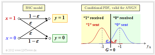
The two shaded areas $($each $\varepsilon)$ mark decision errors under the condition
- $x=0$ ⇒ $\tilde{x} = +1$ (blue),
- $x=1$ ⇒ $\tilde{x} = -1$ (red),
when hard decisions are made:
- \[z = \left\{ \begin{array}{c} 0\\ 1 \end{array} \right.\quad \begin{array}{*{1}c} {\rm if} \hspace{0.15cm} y > 0\hspace{0.05cm},\\ {\rm if} \hspace{0.15cm}y < 0\hspace{0.05cm}.\\ \end{array}\]
For equally probable input symbols, the bit error probability ${\rm Pr}(z \ne x)$ is then also $\varepsilon$. With the "complementary Gaussian error function" ${\rm Q}(x)$ the following holds:
- \[\varepsilon = {\rm Q}(1/\sigma) = {\rm Q}(\sqrt{\rho}) = \frac {1}{\sqrt{2\pi} } \cdot \int_{\sqrt{\rho}}^{\infty}{\rm e}^{- \alpha^2/2} \hspace{0.1cm}{\rm d}\alpha \hspace{0.05cm}.\]
where $\rho = 1/\sigma^2 = 2 \cdot E_{\rm S}/N_0$ denotes the signal–to–noise ratio $\rm (SNR)$ before the decision, using the following system quantities:
- $E_{\rm S}$ is the signal energy per symbol (without coding: $E_{\rm S}=E_{\rm B}$, thus equal to the signal energy per bit),
- $N_0$ denotes the constant (one-sided) noise power density of the AWGN channel.
- Notes: The presented facts are clarified with the $($German language$)$ SWF applet "Symbolfehlerwahrscheinlichkeit von Digitalsystemen"
⇒ "Symbol error probability of digital systems"
Binary Symmetric Channel – BSC
The AWGN channel model is not a digital channel model as we have presupposed in the paragraph "Block diagram and prerequisities" for the introductory description of channel coding methods. However, if we take into account a hard decision, we arrive at the digital model "Binary Symmetric Channel" $\rm (BSC)$:

- We choose the falsification probabilities ${\rm Pr}(y = 1\hspace{0.05cm}|\hspace{0.05cm} x=0)$ resp. ${\rm Pr}(y = 0\hspace{0.05cm}|\hspace{0.05cm} x=1)$ to be
- \[\varepsilon = {\rm Q}(\sqrt{\rho})\hspace{0.05cm}.\]
- Then the connection to the $\text{AWGN}$ channel model is established.
- The decision line is at $G = 0$, which also gives rise to the property "symmetrical".
The BSC model provides a statistically independent error sequence and is thus suitable for modeling memoryless feedback-free channels, which are considered without exception in this book.
For the description of memory-affected channels, other models must be used, which are discussed in the fifth main chapter of the book "Digital Signal Transmission", e.g. "bundle error channels" according to the
$\text{Example 1:}$ The figure shows
- the original image in the middle,
- statistically independent errors according to the BSC model (left),
- so-called "bundle errors" according to Gilbert–Elliott (right).
The bit error rate is $10\%$ in both cases.
From the right graph, it can be seen from the bundle error structure that the image was transmitted line by line.
Binary Erasure Channel – BEC
The BSC model only provides the statements "correct" and "incorrect". However, some receivers – such as the so-called $\text{soft–in soft–out decoder}$ – can also provide some information about the certainty of the decision, although they must of course be informed about which of their input values are certain and which are rather uncertain.
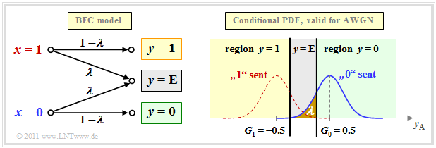
The "Binary Erasure Channel" $\rm (BEC)$ provides such information. On the basis of the graph you can see:
- The input alphabet of the BEC model is binary ⇒ $x ∈ \{0, \hspace{0.05cm}1\}$ and the output alphabet is ternary ⇒ $y ∈ \{0, \hspace{0.05cm}1, \hspace{0.05cm}\rm E\}$.
- An "$\rm E$" denotes an uncertain decision. This new "symbol" stands for "Erasure".
- Bit errors are excluded by the BEC model per se. An unsafe decision $\rm (E)$ is made with probability $\lambda$, while the probability for a correct (and at the same time safe) decision is $1-\lambda$ .
- In the upper right, the relationship between BEC and AWGN model is shown, with the erasure area $\rm (E)$ highlighted in gray.
- In contrast to the BSC model, there are now two decision lines $G_0 = G$ and $G_1 = -G$. It holds:
- \[\lambda = {\rm Q}\big[\sqrt{\rho} \cdot (1 - G)\big]\hspace{0.05cm}.\]
We refer here again to the following applets:
Binary Symmetric Error & Erasure Channel – BSEC
The BEC model is rather unrealistic $($error probability: $0)$ and only an approximation for an extremely large signal–to–noise–power ratio $\rho$.
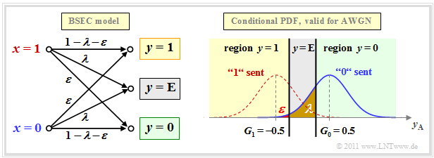
Stronger noise $($a smaller $\rho)$ would be better served by the "Binary Symmetric Error & Erasure Channel" $\rm (BSEC)$ with the two parameters
- Falsification probability $\varepsilon = {\rm Pr}(y = 1\hspace{0.05cm}|\hspace{0.05cm} x=0)= {\rm Pr}(y = 0\hspace{0.05cm}|\hspace{0.05cm} x=1)$,
- Erasure probability $\lambda = {\rm Pr}(y = {\rm E}\hspace{0.05cm}|\hspace{0.05cm} x=0)= {\rm Pr}(y = {\rm E}\hspace{0.05cm}|\hspace{0.05cm} x=1).$
As with the BEC model, $x ∈ \{0, \hspace{0.05cm}1\}$ and $y ∈ \{0, \hspace{0.05cm}1, \hspace{0.05cm}\rm E\}$.
$\text{Example 2:}$ We consider the BSEC model with the two decision lines
- $G_0 = G = 0.5$,
- $G_1 = -G = -0.5$.
The parameters $\varepsilon$ and $\lambda$ are fixed by the $\rm SNR$ $\rho=1/\sigma^2$ of the comparable AWGN channel.
- For $\sigma = 0.5$ ⇒ $\rho = 4$ (assumed for the sketched PDF):
- $$\varepsilon = {\rm Q}\big[\sqrt{\rho} \cdot (1 + G)\big] = {\rm Q}(3) \approx 0.14\%\hspace{0.05cm},$$
- $${\it \lambda} = {\rm Q}\big[\sqrt{\rho} \cdot (1 - G)\big] - \varepsilon = {\rm Q}(1) - {\rm Q}(3) $$
- $$\Rightarrow \hspace{0.3cm}{\it \lambda} \approx 15.87\% - 0.14\% = 15.73\%\hspace{0.05cm},$$
- For $\sigma = 0.25$ ⇒ $\rho = 16$:
- $$\varepsilon = {\rm Q}(6) \approx 10^{-10}\hspace{0.05cm},$$
- $${\it \lambda} = {\rm Q}(2) \approx 2.27\%\hspace{0.05cm}.$$
- Here, the BSEC model could be replaced by the simpler BEC variant without serious differences.
Criteria »Maximum-a-posteriori« and »Maximum-Likelihood«
We now start from the model sketched below and apply the methods already described in chapter "Structure of the optimal receiver" of the book "Digital Signal Transmission" to the decoding process.
$\text{The task of the channel decoder}$
- is to determine the vector $\underline{v}$ so
- that it matches the information word $\underline{u}$ "as well as possible".
Formulated a little more precisely:
- Minimizing the »block error probability«
- $${\rm Pr(block \:error)} = {\rm Pr}(\underline{v} \ne \underline{u}) $$
- related to the vectors $\underline{u}$ and $\underline{v}$ of length $k$ .
- Because of the unique assignment $\underline{x} = {\rm enc}(\underline{u})$ by the channel encoder and $\underline{v} = {\rm enc}^{-1}(\underline{z})$ by the channel decoder applies in the same way:
- \[{\rm Pr(block \:error)} = {\rm Pr}(\underline{z} \ne \underline{x})\hspace{0.05cm}. \]
The channel decoder in the above model consists of two parts:
- The "code word estimator" determines from the received vector $\underline{y}$ an estimate $\underline{z} \in \mathcal{C}$ according to a given criterion.
- From the (received) code word $\underline{z}$ the information word $\underline{v}$ is determined by "simple mapping". This should match $\underline{u}$.
There are a total of four different variants for the code word estimator, viz.
- the maximum–a–posteriori $\rm (MAP)$ receiver for the entire code word $\underline{x}$,
- the maximum–a–posteriori $\rm (MAP)$ receiver for the individual code bits $x_i$,
- the maximum–likelihood $\rm (ML)$ receiver for the entire code word $\underline{x}$,
- the maximum–likelihood $\rm (ML)$ receiver for the individual code bits $x_i$.
Their definitions follow in the next section. First of all, however, the essential distinguishing feature between $\rm MAP$ and $\rm ML$:
$\text{Conclusion:}$
- A MAP receiver, in contrast to the ML receiver, also considers different occurrence probabilities for the entire code word or for their individual bits.
- If all code words $\underline{x}$ and thus all bits $x_i$ of the code words are equally probable, the simpler ML receiver is equivalent to the corresponding MAP receiver.
Definitions of the different optimal receivers
$\text{Definition:}$ The "block–wise maximum–a–posteriori receiver" – for short: »block–wise MAP« – decides among the $2^k$ code words $\underline{x}_i \in \mathcal{C}$ for the code word with the highest a–posteriori probability:
- \[\underline{z} = {\rm arg} \max_{\underline{x}_{\hspace{0.03cm}i} \hspace{0.03cm} \in \hspace{0.05cm} \mathcal{C} } \hspace{0.1cm} {\rm Pr}( \underline{x}_{\hspace{0.03cm}i} \vert\hspace{0.05cm} \underline{y} ) \hspace{0.05cm}.\]
- ${\rm Pr}( \underline{x}_{\hspace{0.03cm}i} \hspace{0.05cm}\vert \hspace{0.05cm} \underline{y} )$ is the "conditional probability" that $\underline{x}_i$ was sent, when $\underline{y}$ is received.
We now try to simplify this decision rule step by step. The inference probability can be transformed according to "Bayes rule" as follows:
- \[{\rm Pr}( \underline{x}_{\hspace{0.03cm}i} \hspace{0.05cm}\vert \hspace{0.05cm} \underline{y} ) = \frac{{\rm Pr}( \underline{y} \hspace{0.08cm} |\hspace{0.05cm} \underline{x}_{\hspace{0.03cm}i} ) \cdot {\rm Pr}( \underline{x}_{\hspace{0.03cm}i} )}{{\rm Pr}( \underline{y} )} \hspace{0.05cm}.\]
- The probability ${\rm Pr}( \underline{y}) $ is independent of $\underline{x}_i$ and need not be considered in maximization.
- Moreover, if all $2^k$ information words $\underline{u}_i$ are equally probable, then the maximization can also dispense with the contribution ${\rm Pr}( \underline{x}_{\hspace{0.03cm}i} ) = 2^{-k}$ in the numerator.
$\text{Definition:}$ The "block–wise maximum–likelihood receiver" – for short: »block–wise ML« – decides among the $2^k$ allowed code words $\underline{x}_i \in \mathcal{C}$ for the code word with the highest transition probability:
- \[\underline{z} = {\rm arg} \max_{\underline{x}_{\hspace{0.03cm}i} \hspace{0.05cm} \in \hspace{0.05cm} \mathcal{C} } \hspace{0.1cm} {\rm Pr}( \underline{y} \hspace{0.05cm}\vert\hspace{0.05cm} \underline{x}_{\hspace{0.03cm}i} ) \hspace{0.05cm}.\]
- The conditional probability ${\rm Pr}( \underline{y} \hspace{0.05cm}\vert\hspace{0.05cm} \underline{x}_{\hspace{0.03cm}i} )$ is now to be understood in the forward direction, namely as the probability that the vector $\underline{y}$ is received when the code word $\underline{x}_i$ has been sent.
- In the following, we always use the maximum–likelihood receiver at the block level. Due to the assumed equally likely information words, this also always provides the best possible decision.
However, the situation is different on the bit level. The goal of an iterative decoding is just to estimate probabilities for all code bits $x_i \in \{0, 1\}$ and to pass these on to the next stage. For this one needs a MAP receiver.
$\text{Definition:}$ The "bit–wise maximum–a–posteriori receiver" – for short: »bit–wise MAP« – selects for each individual code bit $x_i$ the value $(0$ or $1)$ with the highest inference probability ${\rm Pr}( {x}_{\hspace{0.03cm}i}\vert \hspace{0.05cm} \underline{y} )$:
- \[\underline{z} = {\rm arg}\hspace{-0.1cm}{ \max_{ {x}_{\hspace{0.03cm}i} \hspace{0.03cm} \in \hspace{0.05cm} \{0, 1\} } \hspace{0.03cm} {\rm Pr}( {x}_{\hspace{0.03cm}i}\vert \hspace{0.05cm} \underline{y} ) \hspace{0.05cm} }.\]
Maximum-likelihood decision at the BSC channel
We now apply the maximum–likelihood criterion to the memoryless $\text{BSC channel}$. Then holds:
- \[{\rm Pr}( \underline{y} \hspace{0.05cm}|\hspace{0.05cm} \underline{x}_{\hspace{0.03cm}i} ) = \prod\limits_{l=1}^{n} {\rm Pr}( y_l \hspace{0.05cm}|\hspace{0.05cm} x_l ) \hspace{0.5cm}{\rm with}\hspace{0.5cm} {\rm Pr}( y_l \hspace{0.05cm}|\hspace{0.05cm} x_l ) = \left\{ \begin{array}{c} 1 - \varepsilon\\ \varepsilon \end{array} \right.\quad \begin{array}{*{1}c} {\rm if} \hspace{0.15cm} y_l = x_l \hspace{0.05cm},\\ {\rm if} \hspace{0.15cm}y_l \ne x_l\hspace{0.05cm}.\\ \end{array} \hspace{0.05cm}.\]
- \[\Rightarrow \hspace{0.3cm} {\rm Pr}( \underline{y} \hspace{0.05cm}|\hspace{0.05cm} \underline{x}_{\hspace{0.03cm}i} ) = \varepsilon^{d_{\rm H}(\underline{y} \hspace{0.05cm}, \hspace{0.1cm}\underline{x}_{\hspace{0.03cm}i})} \cdot (1-\varepsilon)^{n-d_{\rm H}(\underline{y} \hspace{0.05cm}, \hspace{0.1cm}\underline{x}_{\hspace{0.03cm}i})} \hspace{0.05cm}.\]
$\text{Proof:}$ This result can be justified as follows:
- The $\text{Hamming distance}$ $d_{\rm H}(\underline{y} \hspace{0.05cm}, \hspace{0.1cm}\underline{x}_{\hspace{0.03cm}i})$ specifies the number of bit positions where the words $\underline{y}$ and $\underline{x}_{\hspace{0.03cm}i}$ with each $n$ binary element differ. Example: The Hamming distance between $\underline{y}= (0, 1, 0, 1, 0, 1, 1)$ and $\underline{x}_{\hspace{0.03cm}i} = (0, 1, 0, 0, 1, 1, 1)$ is $2$.
- In $n - d_{\rm H}(\underline{y} \hspace{0.05cm}, \hspace{0.1cm}\underline{x}_{\hspace{0.03cm}i})$ positions thus the two vectors $\underline{y}$ and $\underline{x}_{\hspace{0.03cm}i}$ do not differ. In the above example, five of the $n = 7$ bits are identical.
- Finally, one arrives at the above equation by substituting the falsification probability $\varepsilon$ or its complement $1-\varepsilon$.
The approach to maximum–likelihood decoding is to find the code word $\underline{x}_{\hspace{0.03cm}i}$ that has the transition probability ${\rm Pr}( \underline{y} \hspace{0.05cm}|\hspace{0.05cm} \underline{x}_{\hspace{0.03cm}i} )$ maximized:
- \[\underline{z} = {\rm arg} \max_{\underline{x}_{\hspace{0.03cm}i} \hspace{0.05cm} \in \hspace{0.05cm} \mathcal{C}} \hspace{0.1cm} \left [ \varepsilon^{d_{\rm H}(\underline{y} \hspace{0.05cm}, \hspace{0.1cm}\underline{x}_{\hspace{0.03cm}i})} \cdot (1-\varepsilon)^{n-d_{\rm H}(\underline{y} \hspace{0.05cm}, \hspace{0.1cm}\underline{x}_{\hspace{0.03cm}i})} \right ] \hspace{0.05cm}.\]
Since the logarithm is a monotonically increasing function, the same result is obtained after the following maximization:
- \[\underline{z} = {\rm arg} \max_{\underline{x}_{\hspace{0.03cm}i} \hspace{0.05cm} \in \hspace{0.05cm} \mathcal{C}} \hspace{0.1cm} L(\underline{x}_{\hspace{0.03cm}i})\hspace{0.5cm} {\rm with}\hspace{0.5cm} L(\underline{x}_{\hspace{0.03cm}i}) = \ln \left [ \varepsilon^{d_{\rm H}(\underline{y} \hspace{0.05cm}, \hspace{0.1cm}\underline{x}_{\hspace{0.03cm}i})} \cdot (1-\varepsilon)^{n-d_{\rm H}(\underline{y} \hspace{0.05cm}, \hspace{0.1cm}\underline{x}_{\hspace{0.03cm}i})} \right ] \]
- \[ \Rightarrow \hspace{0.3cm} L(\underline{x}_{\hspace{0.03cm}i}) = d_{\rm H}(\underline{y} \hspace{0.05cm}, \hspace{0.1cm}\underline{x}_{\hspace{0.03cm}i}) \cdot \ln \hspace{0.05cm} \varepsilon + \big [n -d_{\rm H}(\underline{y} \hspace{0.05cm}, \hspace{0.1cm}\underline{x}_{\hspace{0.03cm}i})\big ] \cdot \ln \hspace{0.05cm} (1- \varepsilon) = \ln \frac{\varepsilon}{1-\varepsilon} \cdot d_{\rm H}(\underline{y} \hspace{0.05cm}, \hspace{0.1cm}\underline{x}_{\hspace{0.03cm}i}) + n \cdot \ln \hspace{0.05cm} (1- \varepsilon) \hspace{0.05cm}.\]
Here we have to take into account:
- The second term of this equation is independent of $\underline{x}_{\hspace{0.03cm}i}$ and need not be considered further for maximization.
- Also, the factor before Hamming distance is the same for all $\underline{x}_{\hspace{0.03cm}i}$.
- Since $\ln \, {\varepsilon}/(1-\varepsilon)$ is negative (at least for $\varepsilon <0.5$, which can be assumed without much restriction), maximization becomes minimization, and the following final result is obtained:
$\text{Maximum–likelihood decision at the BSC channel:}$
Choose from the $2^k$ allowed code words $\underline{x}_{\hspace{0.03cm}i}$ the one with the »least Hamming distance« $d_{\rm H}(\underline{y} \hspace{0.05cm}, \hspace{0.1cm}\underline{x}_{\hspace{0.03cm}i})$ to the received vector $\underline{y}$:
- \[\underline{z} = {\rm arg} \min_{\underline{x}_{\hspace{0.03cm}i} \hspace{0.05cm} \in \hspace{0.05cm} \mathcal{C} } \hspace{0.1cm} d_{\rm H}(\underline{y} \hspace{0.05cm}, \hspace{0.1cm}\underline{x}_{\hspace{0.03cm}i})\hspace{0.05cm}, \hspace{0.2cm} \underline{y} \in {\rm GF}(2^n) \hspace{0.05cm}, \hspace{0.2cm}\underline{x}_{\hspace{0.03cm}i}\in {\rm GF}(2^n) \hspace{0.05cm}.\]
Applications of ML/BSC decision can be found in the following sections:
- $\text{SPC}$ $($"single parity–check code"$)$.
- $\text{RC}$ $($"repetition code"$)$.
Maximum-likelihood decision at the AWGN channel
The AWGN model for a $(n, k)$ block code differs from the $\text{model}$ in the first chapter section in that for $x$, $\tilde{x}$ and $y$ now the corresponding vectors $\underline{x}$, $\underline{\tilde{x}}$ and $\underline{y}$ must be used, each consisting of $n$ elements.
The steps to derive the maximum–likelihood decision for AWGN are given below only in bullet form:
- The AWGN channel is memoryless per se (the "White" in the name stands for this). Thus, for the conditional probability density function $\rm (PDF)$, it can be written:
- \[f( \underline{y} \hspace{0.05cm}|\hspace{0.05cm} \underline{\tilde{x}} ) = \prod\limits_{l=1}^{n} f( y_l \hspace{0.05cm}|\hspace{0.05cm} \tilde{x}_l ) \hspace{0.05cm}.\]
- The conditional PDF is "Gaussian" for each individual code element $(l = 1, \hspace{0.05cm}\text{...} \hspace{0.05cm}, n)$. Thus, the entire PDF also satisfies a (one-dimensional) Gaussian distribution:
- \[f({y_l \hspace{0.03cm}| \hspace{0.03cm}\tilde{x}_l }) = \frac {1}{\sqrt{2\pi} \cdot \sigma } \cdot \exp \left [ - \frac {(y_l - \tilde{x}_l)^2}{2\sigma^2} \right ]\hspace{0.3cm} \Rightarrow \hspace{0.3cm} f( \underline{y} \hspace{0.05cm}|\hspace{0.05cm} \underline{\tilde{x}} ) = \frac {1}{(2\pi)^{n/2} \cdot \sigma^n } \cdot \exp \left [ - \frac {1}{2\sigma^2} \cdot \sum_{l=1}^{n} \hspace{0.2cm}(y_l - \tilde{x}_l)^2 \right ] \hspace{0.05cm}.\]
- Since $\underline{y}$ is now value-continuous rather than value-discrete as in the BSC model, probability densities must now be examined according to the maximum-likelihood decision rule rather than probabilities. The optimal result is:
- \[\underline{z} = {\rm arg} \max_{\underline{x}_{\hspace{0.03cm}i} \hspace{0.05cm} \in \hspace{0.05cm} \mathcal{C}} \hspace{0.1cm} f( \underline{y} \hspace{0.05cm}|\hspace{0.05cm} \underline{\tilde{x}}_i )\hspace{0.05cm}, \hspace{0.5cm} \underline{y} \in R^n\hspace{0.05cm}, \hspace{0.2cm}\underline{x}_{\hspace{0.03cm}i}\in {\rm GF}(2^n) \hspace{0.05cm}.\]
- In algebra, the distance between two points $\underline{y}$ and $\underline{\tilde{x}}$ in $n$–dimensional space is called the $\text{Euclidean distance}$, named after the Greek mathematician $\text{Euclid}$ who lived in the third century BC:
- \[d_{\rm E}(\underline{y} \hspace{0.05cm}, \hspace{0.1cm}\underline{\tilde{x}}) = \sqrt{\sum_{l=1}^{n} \hspace{0.2cm}(y_l - \tilde{x}_l)^2}\hspace{0.05cm},\hspace{0.8cm} \underline{y} \in R^n\hspace{0.05cm}, \hspace{0.2cm}\underline{x}_{\hspace{0.03cm}i}\in \mathcal{C} \hspace{0.05cm}.\]
- Thus, the maximum-likelihood decision rule at the AWGN channel for any block code considering that the first factor of the PDF $f( \underline{y} \hspace{0.05cm}|\hspace{0.05cm} \underline{\tilde{x}_i} )$ is constant:
- \[\underline{z} = {\rm arg} \max_{\underline{x}_{\hspace{0.03cm}i} \hspace{0.05cm} \in \hspace{0.05cm} \mathcal{C}} \hspace{0.1cm} \exp \left [ - \frac {d_{\rm E}(\underline{y} \hspace{0.05cm}, \hspace{0.1cm}\underline{\tilde{x}}_i)}{2\sigma^2} \right ]\hspace{0.05cm}, \hspace{0.8cm} \underline{y} \in R^n\hspace{0.05cm}, \hspace{0.2cm}\underline{x}_{\hspace{0.03cm}i}\in {\rm GF}(2^n) \hspace{0.05cm}.\]
- After a few more intermediate steps, you arrive at the result:
$\text{Maximum–likelihood decision at the AWGN channel:}$
Choose from the $2^k$ allowed code words $\underline{x}_{\hspace{0.03cm}i}$ the one with the »smallest Euclidean distance« $d_{\rm E}(\underline{y} \hspace{0.05cm}, \hspace{0.1cm}\underline{x}_{\hspace{0.03cm}i})$ to the received vector $\underline{y}$:
- \[\underline{z} = {\rm arg} \min_{\underline{x}_{\hspace{0.03cm}i} \hspace{0.05cm} \in \hspace{0.05cm} \mathcal{C} } \hspace{0.1cm} d_{\rm E}(\underline{y} \hspace{0.05cm}, \hspace{0.1cm}\underline{x}_{\hspace{0.03cm}i})\hspace{0.05cm}, \hspace{0.8cm} \underline{y} \in R^n\hspace{0.05cm}, \hspace{0.2cm}\underline{x}_{\hspace{0.03cm}i}\in {\rm GF}(2^n) \hspace{0.05cm}.\]
Exercises for the chapter
Exercise 1.3: Channel Models "BSC - BEC - BSEC - AWGN"
Exercise 1.4: Maximum Likelihood Decision


