Contents
- 1 Free distance vs. minimum distance
- 2 Path weighting enumerator function
- 3 Enhanced path weighting enumerator function
- 4 Path weighting enumerator function from state transition diagram
- 5 Rules for manipulating the state transition diagram
- 6 Block error probability vs. burst error probability
- 7 Burst error probability and Bhattacharyya bound
- 8 Bit error probability and Viterbi bound
- 9 Exercises for the chapter
- 10 Quellenverzeichnis
Free distance vs. minimum distance
An important parameter regarding the error probability of linear block codes is the minimum distance between two code words $\underline{x}$ and $\underline{x}\hspace{0.05cm}'$:
- \[d_{\rm min}(\mathcal{C}) = \min_{\substack{\underline{x},\hspace{0.05cm}\underline{x}\hspace{0.05cm}' \hspace{0.05cm}\in \hspace{0.05cm} \mathcal{C} \\ {\underline{x}} \hspace{0.05cm}\ne \hspace{0.05cm} \underline{x}\hspace{0.05cm}'}}\hspace{0.1cm}d_{\rm H}(\underline{x}, \hspace{0.05cm}\underline{x}\hspace{0.05cm}') = \min_{\substack{\underline{x} \hspace{0.05cm}\in \hspace{0.05cm} \mathcal{C} \\ {\underline{x}} \hspace{0.05cm}\ne \hspace{0.05cm} \underline{0}}}\hspace{0.1cm}w_{\rm H}(\underline{x}) \hspace{0.05cm}.\]
The second part of the equation arises from the fact that every linear code also includes the zero word $(\underline{0})$ . It is therefore convenient to set $\underline{x}\hspace{0.05cm}' = \underline{0}$, so that the "Hamming distance" $d_{\rm H}(\underline{x}, \ \underline{0})$ gives the same result as Hamming weight $w_{\rm H}(\underline{x})$.
$\text{Example 1:}$ The table shows the 16 codewords of the "$(7, 4, 3)$ Hamming codes"
$($see $\text{Example 7})$.
- All codewords except the null word $(\underline{0})$ contain at least three ones ⇒ $d_{\rm min} = 3$.
- There are seven codewords with three ones (highlighted in yellow), seven with four ones (highlighted in green), and one each with no ones and seven ones
.
The free distance $d_{\rm F}$ of a (convolutional code ⇒ $\mathcal{CC}$) is formulaically no different from the minimum distance of a linear block code:
- \[d_{\rm F}(\mathcal{CC}) = \min_{\substack{\underline{x},\hspace{0.05cm}\underline{x}\hspace{0.05cm}' \hspace{0.05cm}\in \hspace{0.05cm} \mathcal{CC} \\ {\underline{x}} \hspace{0.05cm}\ne \hspace{0.05cm} \underline{x}\hspace{0.05cm}'}}\hspace{0.1cm}d_{\rm H}(\underline{x}, \hspace{0.05cm}\underline{x}\hspace{0.05cm}') = \min_{\substack{\underline{x} \hspace{0.05cm}\in \hspace{0.05cm} \mathcal{CC} \\ {\underline{x}} \hspace{0.05cm}\ne \hspace{0.05cm} \underline{0}}}\hspace{0.1cm}w_{\rm H}(\underline{x}) \hspace{0.05cm}.\]
In the literature instead of $d_{\rm F}$ sometimes also $d_{∞}$ is used.
- Major difference to minimal distance is that in convolutional codes not information– and codewords are to be considered, but sequences with the property "semi–infinite".
- Each code sequence $\underline{x}$ describes a path through the trellis.
- The free distance is the smallest possible Hamming weight of such a path (except for the zero path).
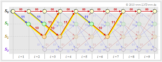
The graph shows three of the infinite paths with the minimum Hamming weight $w_{\rm H, \ min}(\underline{x}) = d_{\rm F} = 5$.
Path weighting enumerator function
For any linear block code, a weight enumerator function can be given in a simple way because of the finite number of codewords $\underline{x}$ . For the $\text{"Example 1"}$ on the previous page this is:
- \[W(X) = 1 + 7 \cdot X^{3} + 7 \cdot X^{4} + X^{7}\hspace{0.05cm}.\]
In the case of a (non terminated) convolutional code, no such weight function can be given, since there are infinitely many, infinitely long code sequences $\underline{x}$ and thus also infinitely many trellis paths. To get a grip on this problem, we now assume the following:
- As a reference for the trellis diagram, we always choose the path of the code sequence $\underline{x} = \underline{0}$ and call this the zero path $\varphi_0$.
- We now consider only those paths $\varphi_j ∈ {\it \Phi}$ that all deviate from the zero path at a given time $t$ and return to it at some point.
Although only a fraction of all paths belong to the set ${\it \Phi}$ , ${\it \Phi} = \{\varphi_1, \ \varphi_2, \ \varphi_3, \ \text{...} \}$ still an unbounded set of paths. $\varphi_0$ is not one of them.
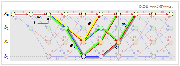
In the above trellis some paths $\varphi_j ∈ {\it \Phi}$ are drawn:
- The yellow path $\varphi_1$ belongs to the sequence $\underline{x}_1 = (11, 10, 11)$ with hamming–weight $w_{\rm H}(\underline{x}_1) = 5$. Thus, the path weighting $w(\varphi_1) = 5$ as well. Due to the definition of the branching time $t$ only this single path $\varphi_1$ has the free distance $d_{\rm F} = 5$ to the zero path ⇒ $A_5 = 1$.
- For the two green paths with corresponding sequences $\underline{x}_2 = (11, 01, 01, 11)$ and $\underline{x}_3 = (11, 10, 00, 10, 11)$ respectively, $w(\varphi_2) = w(\varphi_3) = 6$ holds. No other path exhibits the path weighting $6$ . We take this fact into account by the coefficient $A_6 = 2$.
- Also drawn is the gray path $\varphi_4$, associated with the sequence $\underline{x}_4 = (11, 01, 10, 01, 11)$ ⇒ $w(\varphi_4) = 7$. Also, the sequences $\underline{x}_5 = (11, 01, 01, 00, 10, 11)$, $\underline{x}_6 = (11, 10, 00, 01, 01, 11)$ and $\underline{x}_7 = (11, 10, 00, 10, 00, 10, 11)$ have path weighting $7$ ⇒ $A_7 = 4$.
Thus, the path weighting enumerator function is:
- \[T(X) = A_5 \cdot X^5 + A_6 \cdot X^6 + A_7 \cdot X^7 + \text{...} \hspace{0.1cm}= X^5 + 2 \cdot X^6 + 4 \cdot X^7+ \text{...}\hspace{0.1cm} \hspace{0.05cm}.\]
The definition of this function $T(X)$ is:
$\text{Definition:}$ For the path weighting enumerator function of a convolutional code holds:
- \[T(X) = \sum_{\varphi_j \in {\it \Phi} }\hspace{0.1cm} X^{w(\varphi_j) } \hspace{0.1cm}=\hspace{0.1cm} \sum_{w\hspace{0.05cm} =\hspace{0.05cm} d_{\rm F} }^{\infty}\hspace{0.1cm} A_w \cdot X^w \hspace{0.05cm}.\]
- ${\it \Phi}$ denotes the set of all paths that leave the zero path $\varphi_0$ exactly at the specified time $t$ and return to it (sometime) later.
- According to the second part of the equation, the summands are ordered by their path weightings $w$ where $A_w$ denotes the number of paths with path weighting $w$ .
- The sum starts with $w = d_{\rm F}$.
- The path weighting $w(\varphi_j)$ is equal to the Hamming weight (number of ones) of the code sequence associated to the path $\varphi_j$ $\underline{x}_j$:
- \[w({\varphi_j) = w_{\rm H}(\underline {x} }_j) \hspace{0.05cm}.\]
Note: The weight enumerator function $W(X)$ defined for linear block codes and the path weight function $T(X)$ of convolutional codes have many similarities; however, they are not identical.
We consider again the weight enumerator function of the $(7, 4, 3)$–Hamming code,
- \[W(X) = 1 + 7 \cdot X^{3} + 7 \cdot X^{4} + X^{7},\]
and the path weighting enumerator function of our standard–convolutional coder,
- \[T(X) = X^5 + 2 \cdot X^6 + 4 \cdot X^7+ 8 \cdot X^8+ \text{...} \]
Noticeable is the "$1$" in the first equation, which is missing in the second equation. That is: For the linear block codes, the reference–codeword $\underline{x}_i = \underline{0}$ is counted, whereas the zero code sequence $\underline{x}_i = \underline{0}$ or the zero path $\varphi_0$ is excluded by definition for the convolutional codes.
$\text{Author's personal opinion:}$
One could have defined $W(X)$ without the "$1$" as well. This would have avoided, among other things, that the Bhattacharyya–bound for linear block codes and that for convolutional codes differ by "$-1$", as can be seen from the following equations:
- "Bhattacharyya bound for linear block codes": ${\rm Pr(Block\:error)} \le W(X = \beta) -1 \hspace{0.05cm},$
- "Bhattacharyya bound for convolutional codes": ${\rm Pr(Burst\:error)} \le T(X = \beta) \hspace{0.05cm}.$
Enhanced path weighting enumerator function
The path weighting enumerator function $T(X)$ only provides information regarding the weights of the code sequence $\underline{x}$.
- More information is obtained if the weights of the information sequence $\underline{u}$ are also collected.
- One then needs two formal parameters $X$ and $U$, as can be seen from the following definition.
$\text{Definition:}$ The enhanced path weight enumerator function (EPWEF) is:
- \[T_{\rm enh}(X, U) = \sum_{\varphi_j \in {\it \Phi} }\hspace{0.1cm} X^{w(\varphi_j)} \cdot U^{ { u}(\varphi_j)} \hspace{0.1cm}=\hspace{0.1cm} \sum_{w} \sum_{u}\hspace{0.1cm} A_{w, \hspace{0.05cm}u} \cdot X^w \cdot U^{u} \hspace{0.05cm}.\]
All specifications for $T(X)$–definition on the last page apply. In addition, note:
- The path input weight $u(\varphi_j)$ is equal to the Hamming weight of the information sequence associated to the path $\varphi_j$ $\underline{u}_j$. It is expressed as a power of the formal parameter $U$ .
- The coefficient $A_{w, \ u}$ denotes the number of paths $\varphi_j$ with path output weight $w(\varphi_j)$ and path input weight $u(\varphi_j)$. The run variable for the second portion is $u$ .
- Setting the formal parameter $U = 1$ in the enhanced path weighting enumerator function yields the original weighting enumerator function $T(X)$ according to the definition on the last page.
For many (and all relevant) convolutional codes, upper equation can still be simplified:
- \[T_{\rm enh}(X, U) =\hspace{0.1cm} \sum_{w \ = \ d_{\rm F} }^{\infty}\hspace{0.1cm} A_w \cdot X^w \cdot U^{u} \hspace{0.05cm}.\]
$\text{Example 2:}$ Thus, the enhanced path weighting enumerator function of our standard coder is:
- \[T_{\rm enh}(X, U) = U \cdot X^5 + 2 \cdot U^2 \cdot X^6 + 4 \cdot U^3 \cdot X^7+ \text{ ...} \hspace{0.1cm} \hspace{0.05cm}.\]
If we compare this result with the trellis shown below, we can see:
- The yellow highlighted path – marked by $X^5$ – is composed of a blue arrow $(u_i = 1)$ and two red arrows $(u_i = 0)$ . Thus $X^5$ becomes the extended term $UX^5$.
- The sequences of the two green paths are $\underline{u}_2 = (1, 1, 0, 0)$ ⇒ $\underline{x}_2 = (11, 01, 01, 11)$ and $\underline{u}_3 = (1, 0, 1, 0, 0)$ ⇒ $\underline{x}_3 = (11, 10, 00, 10, 11)$. This gives the second term $2 \cdot U^2X^6$.
- The gray path (and the three undrawn paths) together make the contribution $4 \cdot U^3X^7$. Each of these paths contains three blue arrows ⇒ three ones in the associated information sequence.
Path weighting enumerator function from state transition diagram
There is an elegant way to determine the path weighting enumerator function $T(X)$ and its enhancement directly from the state transition diagram. This will be demonstrated here and on the following pages using our "Standard encoder" as an example.
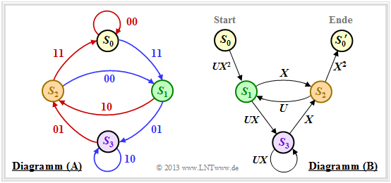
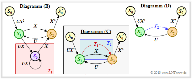
First, the state transition diagram must be redrawn for this purpose. The graphic shows this on the left in the previous form as diagram $\rm (A)$, while the new diagram $\rm (B)$ is given on the right.
It can be seen:
- The state $S_0$ is split into the start state $S_0$ and the end state $S_0\hspace{0.01cm}'$. Thus, all paths of the trellis diagram that start in state $S_0$ and return to it at some point can also be traced in the right graph $\rm (B)$ . Excluded, on the other hand, are direct transitions from $S_0$ to $S_0\hspace{0.01cm}'$ and thus also the zero path $($duration–$S_0)$.
- In the diagram $\rm (A)$ the transitions are distinguishable by the colors red $($for $u_i = 0)$ and blue $($for $u_i = 1)$ and the code words $\underline{x}_i ∈ \{00, 01, 10, 11\}$ are noted at the transitions. In the new diagram $\rm (B)$ are expressed $(00)$ by $X^0 = 1$ and $(11)$ by $X^2$ . The codewords $(01)$ and $(10)$ are now indistinguishable, but are uniformly denoted by $X$ .
- Phrased another way: The codeword $\underline{x}_i$ is now represented as $X^w$ where $X$ is a dummy variable associated with the output (the code sequence); variable and $w = w_{\rm H}(\underline{x}_i)$ indicates the hamming weight of the codeword $\underline{x}_i$ . For a rate $1/2$ code, the exponent $w$ is either $0, \ 1$ or $2$.
- Also the diagram $\rm (B)$ omits the color coding. The information bit $u_i = 1$ is now denoted by $U^1 = U$ and the information bit $u_i = 0$ by $U^0 = 1$ . The dummy–variable $U$ is thus assigned to the input sequence $\underline{u}$ .
Rules for manipulating the state transition diagram
The goal of our calculations will be to characterize the (arbitrarily complicated) path from $S_0$ to $S_0\hspace{0.01cm}'$ by the extended path weighting enumerator function $T_{\rm enh}(X, \ U)$ . For this we need rules to simplify the graph stepwise.
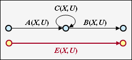
Serial transitions
Two serial connections – denoted by $A(X, \ U)$ and $B(X, \ U)$ – can be replaced by a single connection with the product of these ratings.
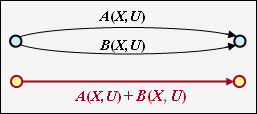
Parallel transitions
Two parallel connections – denoted by $A(X, \ U)$ and $B(X, \ U)$ – are combined by the sum of their valuation functions.
Ring
The adjacent constellation can be replaced by a single connection, and the following applies to the replacement:
- \[E(X, U) = \frac{A(X, U) \cdot B(X, U)}{1- C(X, U)} \hspace{0.05cm}.\]
[[File:P ID2692 KC T 3 5 S3b4.png|right|frame|Reduction of feedback]
Feedback
Due to the feedback, two states can alternate here as often as desired. For this constellation applies:
- \[F(X, U) = \frac{A(X, U) \cdot B(X, U)\cdot C(X, U)}{1- C(X, U)\cdot D(X, U)} \hspace{0.05cm}.\]
The equations for ring and feedback given here are to be proved in the "Exercise 3.12Z" .
$\text{Example 3:}$ The above rules are now to be applied to our standard example. In the graphic on the left you can see the modified diagram $\rm (B)$.
- First we replace the red highlighted detour from $S_1$ to $S_2$ via $S_3$ in the diagram $\rm (B)$ by the red connection drawn in the diagram $\rm (C)$ $T_1(X, \hspace{0.05cm} U)$. According to the upper classification, it is a "ring" with the labels $A = C = U \cdot X$ and $B = X$, and we obtain for the first reduction function:
- \[T_1(X, \hspace{0.05cm} U) = \frac{U \cdot X^2}{1- U \cdot X} \hspace{0.05cm}.\]
- Now we summarize the parallel connections according to the blue background in the diagram $\rm (C)$ and replace it with the blue connection in the diagram $\rm (D)$. The second reduction function is thus:
- \[T_2(X, \hspace{0.05cm}U) = T_1(X, \hspace{0.05cm}U) + X = \frac{U X^2 + X \cdot (1-UX)}{1- U X} = \frac{X}{1- U X} \hspace{0.05cm}.\]
- The entire graph $\rm (D)$ can then be replaced by a single connection from $S_0$ to $S_0\hspace{0.01cm}'$ . According to the feedback rule, one obtains for the enhanced path weighting enumerator function:
- \[T_{\rm enh}(X, \hspace{0.05cm}U) = \frac{(U X^2) \cdot X^2 \cdot \frac{X}{1- U X} }{1- U \cdot \frac{X}{1- U X} } = \frac{U X^5}{1- U X- U X} = \frac{U X^5}{1- 2 \cdot U X} \hspace{0.05cm}.\]
- With the series expansion $1/(1 \, –x) = 1 + x + x^2 + x^3 + \ \text{...} \ $ can also be written for this purpose:
- \[T_{\rm enh}(X, \hspace{0.05cm}U) = U X^5 \cdot \big [ 1 + 2 \hspace{0.05cm}UX + (2 \hspace{0.05cm}UX)^2 + (2 \hspace{0.05cm}UX)^3 + \text{...} \hspace{0.05cm} \big ] \hspace{0.05cm}.\]
- Setting the formal input variable $U = 1$, we obtain the "simple" path weighting enumerator function, which alone allows statements about the weighting distribution of the output sequence $\underline{x}$ :
- \[T(X) = X^5 \cdot \big [ 1 + 2 X + 4 X^2 + 8 X^3 +\text{...}\hspace{0.05cm} \big ] \hspace{0.05cm}.\]
- We have already read the same result from the trellis diagram on page "Path weighting enumerator function" . There was one gray path with weight $5$, two yellow paths with weighting $6$ and four green paths with weighting $7$.
Block error probability vs. burst error probability
The simple model according to the sketch is valid for linear block codes as well as for convolutional codes.
Block codes
For block codes denote $\underline{u} = (u_1, \ \text{...} \hspace{0.05cm}, \ u_i, \ \text{...} \hspace{0.05cm}, \ u_k)$ and $\underline{v} = (v_1, \ \text{...} \hspace{0.05cm}, v_i, \ \text{...} \hspace{0.05cm} \ , \ v_k)$ the information blocks at the input and output of the system.
Thus, the following descriptive variables can be specified:
- the block error probability ${\rm Pr(Block\:error)} = {\rm Pr}(\underline{v} ≠ \underline{u}),$
- the bit error probability ${\rm Pr(Bit\:error)} = {\rm Pr}(v_i ≠ u_i).$
$\text{Please note:}$ In real transmission systems, due to thermal noise, the following always applies:
- $${\rm Pr(Bit\:error)} > 0\hspace{0.05cm},\hspace{1.0cm}{\rm Pr(Block\:error)} > {\rm Pr(Bit\:error)} \hspace{0.05cm}.$$
For this a simple explanation attempt: If the decoder decides in each block of length $k$ exactly one bit wrong,
- so the average bit error probability ${\rm Pr(Bit\:error)}= 1/k$,
- while for the block error probability ${\rm Pr(Block\:error)}\equiv 1$ holds
Convolutional codes
For convolutional codes, the block error probability cannot be specified, since here $\underline{u} = (u_1, \ u_2, \ \text{...} \hspace{0.05cm})$ and $\underline{\upsilon} = (v_1, \ v_2, \ \text{...} \hspace{0.05cm})$ represent sequences.
Even the smallest possible code parameter $k = 1$ here leads to the sequence length $k \hspace{0.05cm}' → ∞$, and the block error probability would always result in ${\rm Pr(block error)}\equiv 1$, even if the bit error probability is extremely small (but non-zero).
$\text{Definition:}$ For the burst error probability of a convolutional code holds:
- \[{\rm Pr(Burst\:error)} = {\rm Pr}\big \{ {\rm Decoder\hspace{0.15cm} leaves\hspace{0.15cm} the\hspace{0.15cm} correct\hspace{0.15cm}path}\hspace{0.15cm}{\rm at\hspace{0.15cm}time \hspace{0.15cm}t}\big \} \hspace{0.05cm}.\]
- To simplify notation for the following derivation, we always assume the zero sequence $(\underline{0})$ which is shown in red in the drawn trellis as the zero path $\varphi_0$ .
- All other paths $\varphi_1, \ \varphi_2, \ \varphi_3, \ \text{...} $ (and many more) leave $\varphi_0$ at time $t$. They all belong to the path set ${\it \Phi}$ ⇒ "Viterbi decoder leaves the correct path at time $t$". This probability is calculated on the next page
.
Burst error probability and Bhattacharyya bound
We proceed as in the earlier chapter "Bounds for block error probability" from the pairwise error probability ${\rm Pr}\big [\varphi_0 → \varphi_i \big]$ that instead of the path $\varphi_0$ the decoder could select the path $\varphi_i$ . All considered paths $\varphi_i$ leave the zero path $\varphi_0$ at time $t$; thus they all belong to the path set ${\it \Phi}$.
The sought burst error probability is equal to the following union set:
- \[{\rm Pr(Burst\:error)}= {\rm Pr}\left (\big[\varphi_{\hspace{0.02cm}0} \mapsto \varphi_{\hspace{0.02cm}1}\big] \hspace{0.05cm}\cup\hspace{0.05cm}\big[\varphi_{\hspace{0.02cm}0} \mapsto \varphi_{\hspace{0.02cm}2}\big]\hspace{0.05cm}\cup\hspace{0.05cm} \text{... }\hspace{0.05cm} \right )= {\rm Pr} \left ( \cup_{\varphi_{\hspace{0.02cm}i} \in {\it \Phi}} \hspace{0.15cm} \big[\varphi_{\hspace{0.02cm}0} \mapsto \varphi_{\hspace{0.02cm}i}\big] \right )\hspace{0.05cm}.\]
An upper bound for this is provided by the so-called "Union bound":
- \[{\rm Pr(Burst\:error)} \le \sum_{\varphi_{\hspace{0.02cm}i} \in {\it \Phi}}\hspace{0.15cm} {\rm Pr}\big [\varphi_{\hspace{0.02cm}0} \mapsto \varphi_{\hspace{0.02cm}i}\big ] = {\rm Pr(Union \hspace{0.15cm}Bound)} \hspace{0.05cm}.\]
The pairwise error probability can be estimated using the "Bhattacharyya bound" :
- \[{\rm Pr}\big [\underline {0} \mapsto \underline {x}_{\hspace{0.02cm}i}\big ] \le \beta^{w_{\rm H}({x}_{\hspace{0.02cm}i})}\hspace{0.3cm}\Rightarrow \hspace{0.3cm} {\rm Pr}\left [\varphi_{\hspace{0.02cm}0} \mapsto \varphi_{\hspace{0.02cm}i}\right ] \le \hspace{0.05cm} \beta^{w(\varphi_i)}\hspace{0.05cm}.\]
Here denotes
- $w_{\rm H}(\underline{x}_i)$ the Hamming weight of the possible code sequence $\underline{x}_i,$
- $\ w(\varphi_i)$ the path weight of the corresponding path $\varphi_i ∈ {\it \Phi}$, and.
- $\beta$ the so-called "Bhattacharyya channel parameter".
By summing over all paths and comparing with the (simple) "path weighting function" $T(X)$ we get the result:
- \[{\rm Pr(Burst\:error)} \le T(X = \beta),\hspace{0.5cm}{\rm mit}\hspace{0.5cm} T(X) = \sum_{\varphi_{\hspace{0.02cm}i} \in {\it \Phi}}\hspace{0.15cm} \hspace{0.05cm} X^{w(\varphi_i)}\hspace{0.05cm}.\]
$\text{Example 4: }$ For our standard encoder ⇒ $R = 1/2, \ m = 2, \ \mathbf{G}(D) = (1 + D + D^2, \ 1 + D)$ we have the following "path weighting enumerator function" obtained:
- \[T(X) = X^5 + 2 \cdot X^6 + 4 \cdot X^7 + \ \text{...} \hspace{0.1cm} = X^5 \cdot ( 1 + 2 \cdot X + 4 \cdot X^2+ \ \text{...} \hspace{0.1cm}) \hspace{0.05cm}.\]
Using the series expansion $1/(1 \, –x) = 1 + x + x^2 + x^3 + \ \text{...} \hspace{0.15cm} $ can also be written for this purpose:
- \[T(X) = \frac{X^5}{1-2 \cdot X} \hspace{0.05cm}.\]
The BSC model provides the following Bhattacharyya bound with the corruption probability $\varepsilon$ :
- \[{\rm Pr(Burst\:error)} \le T(X = \beta) = T\big ( X = 2 \cdot \sqrt{\varepsilon \cdot (1-\varepsilon)} \big ) = \frac{(2 \cdot \sqrt{\varepsilon \cdot (1-\varepsilon)})^5}{1- 4\cdot \sqrt{\varepsilon \cdot (1-\varepsilon)}}\hspace{0.05cm}.\]
In the "Exercise 3.14" this equation is to be evaluated numerically.
Bit error probability and Viterbi bound
Finally, an upper bound is given for the bit error probability. According to the graph, we proceed as in [Liv10][1] assume the following conditions:
- Sent the zero sequence $\underline{x}$ = $\underline{0}$ ⇒ Path $\varphi_0$.
- The duration of a path deviation (error burst duration) is denoted by $L$ .
- The distance between two bursts (inter burst time) we call $N$.
- The hamming weight of the error bundle be $H$.
For a rate–$1/n$–convolutional code ⇒ $k = 1$, i.e., one information bit per clock, the expected values ${\rm E}\big[L \big]$, ${\rm E}\big[N \big]$ and ${\rm E}\big[H\big]$ of the random variables defined above to give an upper bound for the bit error probability:
- \[{\rm Pr(Bit\:error)} = \frac{{\rm E}\big[H\big]}{{\rm E}[L] + {\rm E}\big[N\big]}\hspace{0.15cm} \le \hspace{0.15cm} \frac{{\rm E}\big[H\big]}{{\rm E}\big[N\big]} \hspace{0.05cm}.\]
It is assumed that
- the (mean) duration of a fault burst is in practice much smaller than the expected distance between two bursts,
- the (mean) inter burst time $E\big[N\big]$ is equal to the inverse of the burst fault probability,
- the expected value in the numerator is estimated as follows:
- \[{\rm E}\big[H \big] \le \frac{1}{\rm Pr(Burst\:error)}\hspace{0.1cm} \cdot \sum_{\varphi_{\hspace{0.02cm}i} \in {\it \Phi}}\hspace{0.05cm} \hspace{0.05cm} u(\varphi_i) \cdot \beta^{w(\varphi_i)} \hspace{0.05cm}.\]
In deriving this bound, the pairwise error probability ${\rm Pr}\big [\varphi_0 → \varphi_i \big]$ and the Bhattacharyya estimation are used. Thus one obtains with
- the path input weighting $u(\varphi_i),$
- the path exit weighting $w(\varphi_i),$ and
- the Bhattacharyya parameter $\beta$
we obtain the following estimate for the bit error probability and refer to it as the Viterbi bound:
- \[{\rm Pr(Bit\:error)}\le \sum_{\varphi_{\hspace{0.02cm}i} \in {\it \Phi}}\hspace{0.05cm} \hspace{0.05cm} u(\varphi_i) \cdot \beta^{w(\varphi_i)} \hspace{0.05cm}.\]
This intermediate result can also be represented in another form. We recall the "enhanced path weighting enumerator function"
- \[T_{\rm enh}(X, U) = \sum_{\varphi_j \in {\it \Phi}}\hspace{0.1cm} X^{w(\varphi_j)} \cdot U^{{ u}(\varphi_j)} \hspace{0.05cm}.\]
If we derive this function according to the dummy input variable $U$ , we get
- \[\frac {\rm d}{{\rm d}U}\hspace{0.2cm}T_{\rm enh}(X, U) = \sum_{\varphi_j \in {\it \Phi}}\hspace{0.1cm} { u}(\varphi_j) \cdot X^{w(\varphi_j)} \cdot U^{{ u}(\varphi_j)-1} \hspace{0.05cm}.\]
Finally, if we set $U = 1$ for the dummy–input variable we see the connection to the above result:
- \[\left [ \frac {\rm d}{{\rm d}U}\hspace{0.2cm}T_{\rm enh}(X, U) \right ]_{\substack{ U=1}} = \sum_{\varphi_j \in {\it \Phi}}\hspace{0.1cm} { u}(\varphi_j) \cdot X^{w(\varphi_j)} \hspace{0.05cm}.\]
$\text{Conclusion:}$ The bit error probability of a convolutional code can be estimated using the extended path weighting enumerator function in closed form:
- \[{\rm Pr(Bit\:error)} \le {\rm Pr(Viterbi)} = \left [ \frac {\rm d}{ {\rm d}U}\hspace{0.2cm}T_{\rm enh}(X, U) \right ]_{\substack{X=\beta \\ U=1} } \hspace{0.05cm}.\]
One speaks of the Viterbi bound. Here one derives the enhanced path weighting enumerator function after the second parameter $U$ and then sets
- $X = \beta$,
- $U = 1$.
Note: In "Exercise 3.14" the Viterbi bound and the Bhattacharyya bound for the rate $1/2$ default code and the "BSC–Model" evaluated numerically.
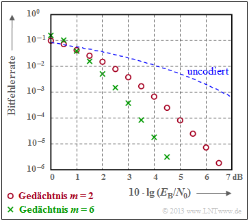
$\text{Example 5:}$ The graph illustrates the good correction capability of the convolutional codes at "AWGN channel".
- Red circles denote the bit error rate for our rate $1/2$ default code with memory $m = 2$.
- Green crosses mark a convolutional code with $m = 6$, the so-called "industry standard code".
In particular, codes with large memory $m$ lead to large gains over uncoded transmission (dashed curve).
Exercises for the chapter
Aufgabe 3.12: Pfadgewichtsfunktion
Aufgabe 3.12Z: Ring und Rückkopplung
Aufgabe 3.13: Nochmals zu den Pfadgewichtsfunktionen
Aufgabe 3.14: Fehlerwahrscheinlichkeitsschranken
Quellenverzeichnis
- ↑ Liva, G.: Channel Coding. Lecture manuscript, Chair of Communications Engineering, TU Munich and DLR Oberpfaffenhofen, 2010.

