Difference between revisions of "Digital Signal Transmission/Error Probability with Intersymbol Interference"

Revision as of 13:25, 17 May 2022

Gaussian receiver filter

We start from the sketched block diagram. The following configuration is assumed for quantitative consideration of the intersymbol interference:

Rectangular NRZ basic transmission pulse $g_s(t)$ with height $s_0$ and duration $T$,
Gaussian-shaped receiver filter with cutoff frequency $f_{\rm G}$ (Note: In this section, we often also denote the exponential function by $\rm exp [ . ]$):

$$H_{\rm E}(f) = H_{\rm G}(f) = {\rm exp}\left [- \frac{\pi \cdot f^2}{(2f_{\rm G})^2} \right ] \hspace{0.2cm} \bullet\!\!-\!\!\!-\!\!\!-\!\!\circ \hspace{0.2cm}h_{\rm E}(t) = h_{\rm G}(t) = {\rm exp}\left [- \pi \cdot (2 f_{\rm G} t)^2\right ] \hspace{0.05cm}.$$

AWGN channel, that is, $H_{\rm K}(f) = 1 $ and ${\it \Phi}_n(f) = N_0/2$.

Block diagram for the chapter "Error probability for intersymbol interference"

Based on the assumptions made here, the following holds for the basic detection pulse:

$$g_d(t) = g_s(t) \star h_{\rm G}(t) = 2 f_{\rm G} \cdot s_0 \cdot \int_{t-T/2}^{t+T/2} {\rm e}^{- \pi \hspace{0.05cm}\cdot\hspace{0.05cm} (2 \hspace{0.05cm}\cdot\hspace{0.05cm} f_{\rm G}\hspace{0.05cm}\cdot\hspace{0.05cm} \tau )^2} \,{\rm d} \tau \hspace{0.05cm}.$$

The integration leads to the following equivalent results:

$$g_d(t) = s_0 \cdot \big [ {\rm Q} \left ( 2 \cdot \sqrt {2 \pi} \cdot f_{\rm G}\cdot ( t - {T}/{2})\right )- {\rm Q} \left ( 2 \cdot \sqrt {2 \pi} \cdot f_{\rm G}\cdot ( t + {T}/{2} )\right ) \big ],$$

$$g_d(t) = s_0 \cdot\big [ {\rm erfc} \left ( 2 \cdot \sqrt {\pi} \cdot f_{\rm G}\cdot ( t - {T}/{2})\right )- {\rm erfc} \left ( 2 \cdot \sqrt {\pi} \cdot f_{\rm G}\cdot ( t + {T}/{2} )\right ) \big ]\hspace{0.05cm}.$$

Here, two variants of the complementary Gaussian error function are used, viz.

$${\rm Q} (x) = \frac{\rm 1}{\sqrt{\rm 2\pi}}\int_{\it x}^{+\infty}\rm e^{\it -u^{\rm 2}/\rm 2}\,d {\it u} \hspace{0.05cm},\hspace{0.5cm} {\rm erfc} (\it x) = \frac{\rm 2}{\sqrt{\rm \pi}}\int_{\it x}^{+\infty}\rm e^{\it -u^{\rm 2}}\,d \it u \hspace{0.05cm}.$$

The module Complementary Gaussian Error Functions provides the numerical values of ${\rm Q} (x)$ and $0.5 \cdot {\rm erfc} (x)$.

The noise power at the output of the Gaussian receiver filter $H_{\rm G}(f)$ is equal to

$$\sigma_d^2 = \frac{N_0}{2} \cdot \int_{-\infty}^{+\infty} |H_{\rm G}(f)|^2 \,{\rm d} f = \frac{N_0\cdot f_{\rm G}}{\sqrt{2}}\hspace{0.05cm}.$$

From these two equations one can already see:

The smaller the cutoff frequency $f_{\rm G}$ of the Gaussian low-pass filter, the smaller the noise rms value $\sigma_d$ and consequently the better the noise performance.

However, a small cutoff frequency leads to a strong deviation of the basic detection pulse $g_d(t)$ from the square wave form and thus to intersymbol interference.

$\text{Example 1:}$ The left graph shows the basic detection pulse $g_d(t)$ at the output of a Gaussian low-pass filter $H_{\rm G}(f)$ with the cutoff frequency $f_{\rm G}$ when an NRZ rectangular pulse (blue curve) is applied at the input.

Basic pulse and noise power density with Gaussian receiver filter

One can see from this plot:

The Gaussian low-pass filter $H_{\rm G}(f)$ causes the detection pulse $g_d(t)$ to be reduced and broadened compared to the transmitted pulse $g_s(t)$ ⇒ time dispersion.

This pulse deformation is the stronger, the smaller the cutoff frequency $f_{\rm G}$ is. For example, with $f_{\rm G} \cdot T = 0.4$ (red curve) the pulse maximum is already reduced to about $68\%$.

In the limiting case $f_{\rm G} \to \infty$ the Gaussian low-pass has no effect ⇒ $g_d(t) = g_s(t)$. However, in this case, no noise limitation is effective at all, as can be seen from the right figure.

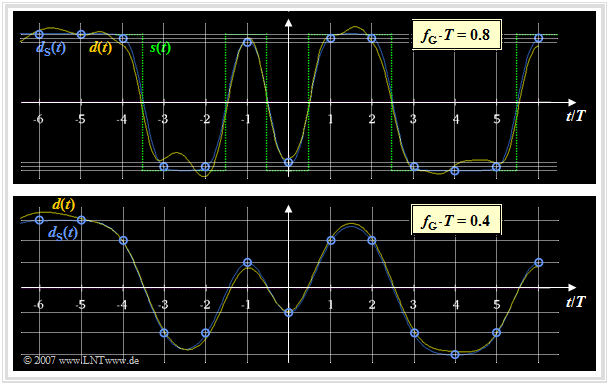
$\text{Example 2:}$ The same preconditions apply as for the last example. The graph shows the detection signal $d(t)$ after the Gaussian low-pass (before the decision) for two different cutoff frequencies, namely $f_{\rm G} \cdot T = 0.8$ and $f_{\rm G} \cdot T = 0.4$

Detection signal with Gaussian receiver filter

Shown equally in both diagrams (but admittedly difficult to see as a screen capture) are:

the component $d_{\rm S}(\nu \cdot T)$ without considering the noise (blue circles at the detection times),
the total detection signal $d(t)$ including the noise component (yellow),
the transmitted signal $s(t)$ as reference signal (green dotted in the upper graph; equally valid for the lower graph).

By comparing these images, the following statements can be verified:

With the cutoff frequency $f_{\rm G} \cdot T = 0.8$ (upper graph), only minorintersymbol interferences result at the detection times $($at multiples of $T)$. Due to the Gaussian low-pass here primarily the corners of the transmitted signal $s(t)$ are rounded.
In contrast, in the lower image $(f_{\rm G} \cdot T = 0.4)$ the effects of the intersymbol interferences are clearly visible. At the detection times $(\nu \cdot T)$, the signal component of the detection signal $d_{\rm S}(\nu \cdot T)$ shown in blue can assume six different values (grid lines drawn).
The noise component $d_{\rm N}(t)$ – recognizable as the difference between the yellow curve and the blue circles – is statistically larger on average with $f_{\rm G} \cdot T = 0.8$ than with $f_{\rm G} \cdot T = 0.4$.
This result can be explained by the right graph of $\text{example 1}$, which shows the power-spectral density of the noise component $d_{\rm N}(t)$:

$${\it \Phi}_{d{\rm N} }(f) = {N_0}/{2} \cdot \vert H_{\rm G}(f) \vert^2 = {N_0}/{2} \cdot {\rm exp}\left [- \frac{2\pi f^2}{(2f_{\rm G})^2} \right ] .$$

The integral over ${\it \Phi}_{d{\rm N} }(f)$ – i.e. the noise power $\sigma_d^2$ – is twice as large for $f_{\rm G} \cdot T = 0.8$ (purple curve) than with $f_{\rm G} \cdot T = 0.4$ (red curve).

Definition and statements of the eye diagram

The above mentioned facts can also be explained by the eye diagram.

$\text{Definition:}$ The eye diagram (or eye pattern) is the sum of all superimposed sections of the detection signal, whose duration is an integer multiple of the symbol duration $T$.

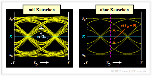
$\text{Example 3:}$ We assume a redundancy-free binary bipolar NRZ rectangular signal $s(t)$ and the Gaussian low-pass filter with cutoff frequency $f_{\rm G} \cdot T = 0.4$.

Eye diagrams with and without noise

Shown are the eye diagrams after the Gaussian low-pass,

left with noise ⇒ signal $d(t)$,
on the right without taking noise into account ⇒ signal $d_{\rm S}(t)$.

This diagram has a certain resemblance to an eye, which led to its naming.
This representation allows important statements about the quality of a digital transmission system:

Only the eye diagram of the signal $d(t)$ can be displayed metrologically on an oscilloscope, which is triggered with the clock signal. From this eye diagram (left graph), for example, the noise rms value $\sigma_d$ can be read – or rather: estimated – werden.

The eye diagram without noise (right graph) refers to the signal component of the detection signal $d_{\rm S}(t)$ and can only be determined by means of a computer simulation. For an implemented system, this eye diagram cannot be displayed, since the noise component $d_{\rm N}(t)$ cannot be eliminated.

In both diagrams, $2048$ eye lines were drawn in each case. In the right graph, however, only $2^5 = 32$ eye lines are distinguishable because the present basic transmitter pulse $g_d(t)$ is limited to the time range $\vert t\vert \le 2T$ (see graph in example 1 with $f_{\rm G} \cdot T = 0.4$, red curve).

The inner eye lines determine the vertical eye opening $\ddot{o}(T_{\rm D})$. The smaller this is, the greater is the influence of intersymbol interference. For a (intersymbol interference free) Nyquist system the vertical eye opening is maximum. Normalized to the transmitted amplitude, $\ddot{o}(T_{\rm D})/s_0 = 2$ is then valid.

With symmetrical basic pulse, the detection time $T_{\rm D} = 0$ is optimal. With a different value $($for example $T_{\rm D} = T/10) $, $\ddot{o}(T_{\rm D})$ would be somewhat smaller and thus the error probability would be significantly larger. This case is indicated by the purple–dashed vertical line in the right graph.

Mean error probability

As with the previous graphs in this chapter, we assume the following:

NRZ rectangles with amplitude $s_0$, AWGN noise with $N_0$, where

$$10 \cdot {\rm lg}\hspace{0.1cm} \frac{s_0^2 \cdot T}{N_0}\approx 13\,{\rm dB}\hspace{0.3cm}\Rightarrow \hspace{0.3cm} \frac{N_0}{s_0^2 \cdot T} = 0.05\hspace{0.05cm}.$$

Gaussian receiver filter with cutoff frequency $f_{\rm G} \cdot T = 0.4$:

$$\sigma_d^2 = \frac{(N_0 /T)\cdot (f_{\rm G}\cdot T)}{\sqrt{2}}= \frac{0.05 \cdot s_0^2\cdot0.4}{\sqrt{2}} \hspace{0.3cm} \Rightarrow \hspace{0.3cm} \sigma_d = \sqrt{0.0141}\cdot s_0 \approx 0.119 \cdot s_0 \hspace{0.05cm}.$$

Let $g_d(\nu \cdot T) \approx 0$ be valid for $|\nu| \ge 2$. The other basic detection pulse values are given as follows:

$$g_0 = g_d(t=0) \approx 0.68 \cdot s_0, \hspace{0.5cm}g_1 = g_d(t=T) \approx 0.16 \cdot s_0, \hspace{0.2cm} g_{-1} = g_d(t=-T) \approx 0.16 \cdot s_0\hspace{0.05cm}.$$

Eye diagram and PDF of the signal component

Let us now analyze the possible values for the signal component of the detection signal $d_{\rm S}(t)$ at the detection times:

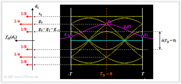
Of the total $32$ eye lines, four lines intersect the ordinate $(t = 0)$ at $g_0 + 2 \cdot g_1 = s_0$. These lines belong to the amplitude coefficients "$\text{...}\hspace{0.05cm} +\hspace{-0.1cm}1,\hspace{0.05cm} {\it +\hspace{-0.05cm}1},\hspace{0.05cm} +\hspace{-0.05cm}1\hspace{0.05cm} \text{...}$". Here, the "middle" coefficient $a_{\nu = 0}$ is highlighted in italics.
The four eye lines, each representing the coefficients "$\text{...}\hspace{0.05cm} -\hspace{-0.1cm}1,\hspace{0.05cm} {\it +\hspace{-0.05cm}1},\hspace{0.05cm} -\hspace{-0.05cm}1,\hspace{0.05cm} \text{...}$" result in the useful sample $d_{\rm S}(T_{\rm D} = 0) =g_0 - 2 \cdot g_1 = 0.36 \cdot s_0$.
In contrast, the useful sample $d_{\rm S}(T_{\rm D} = 0) =g_0 = 0.68 \cdot s_0$ occurs twice as often. This goes back either to the coefficients "$\text{...}\hspace{0.05cm} +\hspace{-0.1cm}1,\hspace{0.05cm} {\it +\hspace{-0.05cm}1},\hspace{0.05cm} -\hspace{-0.05cm}1\hspace{0.05cm} \text{...}$" or to "$\text{...}\hspace{0.05cm} -\hspace{-0.1cm}1,\hspace{0.05cm} {\it +\hspace{-0.05cm}1},\hspace{0.05cm} +\hspace{-0.05cm}1\hspace{0.05cm} \text{...}$".
For the $16$ eye lines which intersect the ordinate $T_{\rm D} = 0$ below the decision threshold $E = 0$, exactly mirror-image relations result.

The possible values $d_{\rm S}(T_{\rm D})$ and their occurrence probabilities can be found in the above graph on the left side in the probability density function (PDF) of the detection useful samples:

$$f_{d{\rm S}}(d_{\rm S}) = {1}/{8} \cdot \delta (d_{\rm S} - s_0)+ {1}/{4} \cdot \delta (d_{\rm S} - 0.68 \cdot s_0)+ {1}/{8} \cdot \delta (d_{\rm S} - 0.36 \cdot s_0)+ $$

$$\hspace{2.15cm} + \hspace{0.2cm} {1}/{8} \cdot \delta (d_{\rm S} + s_0)+{1}/{4} \cdot \delta (d_{\rm S} + 0.68 \cdot s_0)+{1}/{8} \cdot \delta (d_{\rm S} + 0.36 \cdot s_0)\hspace{0.05cm}.$$

Thus, the (average) symbol error probability of the intersymbol interference free system can be given. Taking advantage of the symmetry, one obtains with $\sigma_d/s_0 = 0.119$:

$$p_{\rm S} = {1}/{4} \cdot {\rm Q} \left( \frac{s_0}{ \sigma_d} \right)+ {1}/{2} \cdot {\rm Q} \left( \frac{0.68 \cdot s_0}{ \sigma_d} \right)+{1}/{4} \cdot {\rm Q} \left( \frac{0.36 \cdot s_0}{ \sigma_d} \right)$$

$$\Rightarrow \hspace{0.3cm}p_{\rm S} \approx {1}/{4} \cdot {\rm Q}(8.40) +{1}/{2} \cdot {\rm Q}(5.71)+ {1}/{4} \cdot {\rm Q}(3.02)\approx {1}/{4} \cdot 2.20 \cdot 10^{-17}+ {1}/{2} \cdot 1.65 \cdot 10^{-9}+ {1}/{4} \cdot 1.26 \cdot 10^{-3} \approx 3.14 \cdot 10^{-4} \hspace{0.05cm}.$$

$\text{Conclusion:}$ On the basis of this numerical example one recognizes:

In the presence of intersymbol interference, the (average) symbol error probability $p_{\rm S}$ is essentially determined by the inner eye lines.

The computational cost of determining the error probability $p_{\rm S}$ can become very large, especially if the intersymbol interference comes from very many basic pulse values $g_\nu$.

$\text{Example 4:}$

If the basic pulse values $g_{-5}, \text{...} \ , g_{+5}$ are different from zero and $E \ne 0$, an averaging over $p_{\rm S}$ eye lines is necessary to determine the error probability $2^{11} = 2048$.
If, on the other hand, only the basic pulse values $g_{-1}, \ g_0, \ g_{+1}$ are different from zero and, in addition, the symmetry with respect to the threshold $E = 0$ is taken into account, the effort is reduced to averaging over four terms.
If, in addition, the symmetry $g_{-1} = g_{+1}$ applies as with the above numerical values, then the symmetry with respect to $T_{\rm D}$ can also be exploited and averaging over three terms is sufficient.

Worst-case error probability

In the past, a variety of approximations for the average error probability have been given, among others:

$\text{Definition:}$ As a very simple approximation for the actual error probability $p_{\rm S}$, the worst-case error probability

Relationship between mean and worst-case error probability

$$p_{\rm U} = {\rm Q} \left( \frac{\ddot{o}(T_{\rm D})/2}{ \sigma_d} \right) \hspace{0.05cm}$$ is often used.

For their calculation, the worst-case symbol sequences are always assumed. This means:

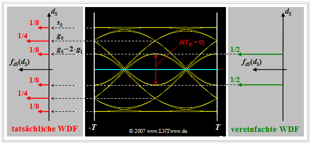
The actual PDF of the useful samples (left graph: six red Diracs) is replaced by a simplified PDF with only the inner Dirac delta functions (right graph: two green Diracs).

For the half vertical eye opening, with the basic pulse values $g_\nu = g_d( T_{\rm D}+ \nu \cdot T)$ generally holds:

$$\ddot{o}(T_{\rm D})/{ 2}= g_0 - \sum_{\nu = 1}^{n} \vert g_{\nu} \vert- \sum_{\nu = 1}^{v} \vert g_{-\nu} \vert \hspace{0.05cm}.$$

This equation can be interpreted as follows:

$g_0 = g_d( T_{\rm D})$ is the so-called main value of the basic pulse. For Nyquist systems $\ddot{o}(T_{\rm D})/{ 2}= g_0$ is always valid. In the following (mostly) $T_{\rm D}= 0$ is set.
The first sum describes the intersymbol interferences of the $n$ trailing pulses of preceding pulses. Tacitly assumed is $g_\nu = 0$ for $\nu \gt n$.
The second sum considers the influence of the $v$ leading pulses of following pulses under the condition $g_{-\nu} = 0$ for $\nu \gt v$.
If all leading and trailing pulses are positive, the two worst-case symbol sequences are "$\text{...}\hspace{0.05cm} -\hspace{-0.1cm}1,\hspace{0.05cm} -\hspace{-0.05cm}1,\hspace{0.05cm} {\it +\hspace{-0.05cm}1},\hspace{0.05cm} -\hspace{-0.05cm}1,\hspace{0.05cm} -\hspace{-0.05cm}1\hspace{0.05cm} \text{...}$" and "$\text{...}\hspace{0.05cm} +\hspace{-0.1cm}1,\hspace{0.05cm} +\hspace{-0.05cm}1,\hspace{0.05cm} {\it -\hspace{-0.05cm}1},\hspace{0.05cm} +\hspace{-0.05cm}1,\hspace{0.05cm} +\hspace{-0.05cm}1\hspace{0.05cm} \text{...}$" (the coefficient $a_{\nu = 0}$ is in italics in each case). These specifications apply, for example, to the Gaussian receiver filter considered here.
If some basic pulse values are negative, this is taken into account in the above equation by the magnitude formation. This results in other "worst–case" sequences than those just mentioned.

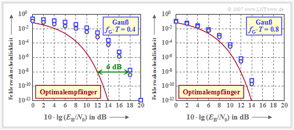
$\text{Example 5:}$ The graph shows the error probabilities of the AWGN channel as a function of the (logarithmized) quotient $E_{\rm B}/N_0$, namely

the average error probability $p_{\rm S}$ with a Gaussian receive filter (blue circles),
the worst-case error probability $p_{\rm U}$ with Gaussian receiver filter (blue rectangles),
the smallest possible error probability according to the section Optimal binary receiver (red curve).

Here, the energy per bit is equal to $E_{\rm B} = s_0^2 \cdot T$ (NRZ rectangular transmitted pulses).

Mean and worst-case error probability vs. $E_{\rm B}/N-0$

The left graph is for the (normalized) cutoff frequency $f_{\rm G} \cdot T = 0.4$, the right one for a broader band receiver filter with $f_{\rm G} \cdot T = 0.8$. The results can be interpreted as follows:

The worst-case error probability $p_{\rm U}$ is always an upper bound for the actual symbol error probability $p_{\rm S}$. The smaller the influence of the intersymbol interference (large cutoff frequency), the closer $p_{\rm S}$ and $p_{\rm U}$ are to each other. For the optimal receiver $p_{\rm S} = p_{\rm U}.$
For Gaussian receiver filter with $f_{\rm G} \cdot T \ge 0.3$, the intersymbol interferences are caused by the neighboring pulses alone $(g_2 = g_3 = \text{...} \approx 0)$, so that a lower bound can also be given for $p_{\rm S}$:

$${p_{\rm U} }/{ 4} \le p_{\rm S} \le p_{\rm U} \hspace{0.05cm}.$$

The strong intersymbol interference of a Gaussian receiver filter with $f_{\rm G} \cdot T = 0.4$ leads to the fact that compared to the optimal receiver a $6 \ \rm dB$ larger $E_{\rm B}/N_0$ must be applied (four times the power), so that the error probability does not exceed the value $10^{-8}$.
However, the horizontal distance between the blue $p_{\rm S}$ curve (marked by circles) and the red comparison curve is not constant. At $p_{\rm S} = 10^{-2}$ the distance is only $4 \ \rm dB$.
The right graph shows that with $f_{\rm G} \cdot T = 0.8$ the distance to the comparison system is less than $1 \ \rm dB$. In the next section it is shown that with a Gaussian receiver filter the (normalized) cutoff frequency $f_{\rm G} \cdot T \approx 0.8$ is the optimum.

Optimization of the cutoff frequency

SNR as a function of the cutoff frequency of a Gaussian low-pass filter

For system optimization and system comparison, it turns out to be convenient,

instead of worst-case error probability $p_{\rm U}$
to use the worst–case signal–to–noise power ratio (S/N ratio):

$$\rho_{\rm U} = [\ddot{o}(T_{\rm D})]^2/ \sigma_d^2.$$

In the case of Gaussian perturbation, the following relationship exists:

$$p_{\rm U} = {\rm Q} \left( \sqrt{\rho_{\rm U}} \right) \hspace{0.05cm}.$$

The mean symbol error probability $p_{\rm S}$ can also be formally expressed by a S/N ratio via the Q function:

$$\rho_d = \left[{\rm Q}^{-1} \left( p_{\rm S} \right)\right]^2 \hspace{0.05cm}.$$

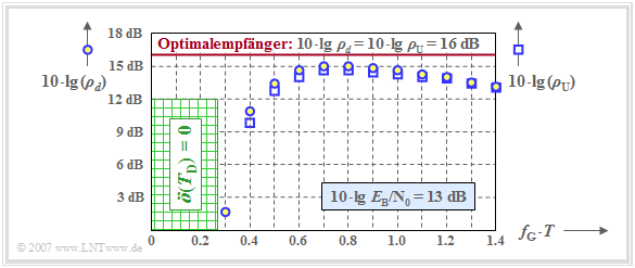
The graph shows the two quantities $\rho_d$ and $\rho_{\rm U}$ in logarithmic form depending on the normalized cutoff frequency $f_{\rm G} \cdot T$ of a Gaussian receiver filter, where $10 \cdot {\rm lg}\hspace{0.1cm} E_{\rm B}/N_0 = 13 \ \rm dB$ is the basis.

The circles outlined in blue are for $10 \cdot {\rm lg}\hspace{0.1cm} \rho_d$ ⇒ "mean" detection SNR,
The blue outlined squares mark $10 \cdot {\rm lg}\hspace{0.1cm} \rho_{\rm U}$ ⇒ "worst-case" SNR.

For comparison, the result for the optimal binary receiver is also plotted as a red horizontal line. For this one holds:

$$\rho_d = \rho_{\rm U} = {2 \cdot E_{\rm B}}/{ N_0}\hspace{0.3cm}\Rightarrow \hspace{0.3cm} 10 \cdot {\rm lg}\hspace{0.1cm} \rho_d = 10 \cdot {\rm lg}\hspace{0.1cm} \rho_{\rm U} \approx 16\,{\rm dB} \hspace{0.05cm}.$$

One can see from the plot:

The optimization criterion $\rho_d$ leads to the optimal cutoff frequency $f_\text{G, opt} \cdot T = 0.8$. A smaller cutoff frequency results in stronger intersymbol interference (smaller eye opening), a larger cutoff frequency results in a larger noise rms value $\sigma_d$.
Such a Gaussian receiver filter with $f_\text{G, opt} \cdot T \approx 0.8$ leads to the signal-to-noise ratio $10 \cdot {\rm lg}\hspace{0.1cm} \rho_d \approx 15 \ \rm dB$ and thus to the error probability $p_{\rm S} \approx 10^{-8}$. For comparison: For the optimal receiver (impulse response matched to the transmitter), the results are $10 \cdot {\rm lg}\hspace{0.1cm} \rho_d \approx 16 \ \rm dB$ and $p_{\rm S} \approx 10^{-10}$.
However, the graph also shows that the much simpler optimization criterion $ \rho_{\rm U}$ $($or $ p_{\rm U})$ leads approximately to the same optimal cutoff frequency $f_\text{G, opt} \cdot T = 0.8$. For this cutoff frequency, we obtain $10 \cdot {\rm lg}\hspace{0.1cm} \rho_{\rm U} \approx 14.7 \ \rm dB$ and the worst-case error probability $p_{\rm U} \approx 3 \cdot 10^{-8}$.
If the cutoff frequency $f_\text{G} \cdot T < 0.27$, the vertical eye opening will always be $\ddot{o}(T_{\rm D}) = 0$. This is called a closed eye. As a consequence, some worst-case pulse sequences would always be wrongly decided even without noise. A systematic error occurs.
Further investigations have shown that the optimization criterion $ \rho_{\rm U}$ is sufficient even with smaller $E_{\rm B}/N_0$. Thus, for a distortion-free channel ⇒ $H_{\rm K}(f) = 1$, the optimal cutoff frequency of the Gaussian low-pass always results in $f_\text{G, opt} \cdot T \approx 0.8$, at least in a realistic approach.

All statements of this chapter can be reproduced with the interactive applet Eye diagram and eye opening.

Exercises for the chapter

Exercise 3.2: Eye Pattern according to Gaussian Low-Pass

Exercise 3.2Z: Optimum Cut-off Frequency for Gaussian Low-pass

@@ Line 8: / Line 8: @@
 == Gaussian receiver filter==
 <br>
-We start from the sketched block diagram. The following configuration is assumed for quantitative consideration of the &nbsp;[[Digital_Signal_Transmission/Ursachen_und_Auswirkungen_von_Impulsinterferenzen#Definition_des_Begriffs_.E2.80.9EImpulsinterferenz.E2.80.9D|intersymbol interference]]:&nbsp;
+We start from the sketched block diagram. The following configuration is assumed for quantitative consideration of the &nbsp;[[Digital_Signal_Transmission/Causes_and_Effects_of_Intersymbol_Interference#Definition_of_the_term_.22Intersymbol_Interference.22|intersymbol interference]]:&nbsp;
 *Rectangular NRZ basic transmission pulse &nbsp;$g_s(t)$&nbsp; with height &nbsp;$s_0$&nbsp; and duration &nbsp;$T$,<br>
 *Gaussian-shaped receiver filter with cutoff frequency &nbsp;$f_{\rm G}$ &nbsp;(''Note:'' &nbsp; In this section, we often also denote the exponential function by &nbsp;$\rm exp [ . ]$):