Exercise 3.5: Kullback-Leibler Distance and Binomial Distribution

• Return to book

Given probabilities

We assume here the  binomial distribution , which is characterised by the parameters  $I$  and  $p$   
⇒   see the book "Stochastische Signaltheorie":

• Range of Values:

$$X = \{\hspace{0.05cm}0\hspace{0.05cm}, \hspace{0.15cm} 1\hspace{0.05cm},\hspace{0.15cm} 2\hspace{0.05cm},\hspace{0.15cm} \text{...}\hspace{0.1cm} ,\hspace{0.15cm} {\mu}\hspace{0.05cm}, \hspace{0.05cm}\text{...}\hspace{0.1cm} , \hspace{0.15cm} I\hspace{0.05cm}\}\hspace{0.05cm},$$

• Probabilities:

$$P_X (X = \mu) = {I \choose \mu} \cdot p^{\mu} \cdot (1-p)^{I-\mu} \hspace{0.05cm},$$

• Linear mean:

$$m_X = I \cdot p \hspace{0.05cm},$$

• Variance:

$$\sigma_X^2 = I \cdot p \cdot (1-p)\hspace{0.05cm}.$$

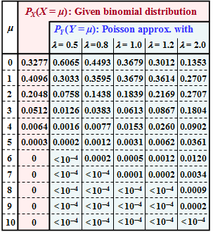
In the part of the table highlighted in red, the probabilities  $P_X(X = \mu$)  of the binomial distribution under consideration are given.  In subtask  (1)  you are to determine the corresponding distribution parameters  $I$  and  $p$ .

This given binomial distribution is to be approximated here by a  Poisson distribution  $Y$ , characterised by the rate  $\lambda$:

• Range of values:

$$Y = \{\hspace{0.05cm}0\hspace{0.05cm}, \hspace{0.15cm} 1\hspace{0.05cm},\hspace{0.05cm} 2\hspace{0.05cm},\hspace{0.15cm} \text{...}\hspace{0.1cm} ,\hspace{0.15cm} {\mu}\hspace{0.05cm}, \hspace{0.05cm}\text{...}\hspace{0.1cm}\}\hspace{0.05cm},$$

• Probabilites:

$$P_Y (Y = \mu) = \frac{\lambda^{\mu}}{\mu !} \cdot {\rm e}^{\lambda} \hspace{0.05cm},$$

• Expected values:

$$m_Y = \sigma_Y^2 = \lambda\hspace{0.05cm}.$$

In order to assess whether the probability function  $P_X(X)$  is sufficiently well approximated by  $P_Y(Y)$ , one can resort to the so-called  Kullback–Leibler distances  (KLD)  , sometimes also called  "relative entropies"  in the literature.

Adapted to the present example, these are:

$$D(P_X \hspace{0.05cm}|| \hspace{0.05cm} P_Y) \hspace{0.15cm} = \hspace{0.15cm} {\rm E} \left [ {\rm log}_2 \hspace{0.1cm} \frac{P_X(X)}{P_Y(X)}\right ] \hspace{0.2cm}=\hspace{0.2cm} \sum_{\mu = 0}^{I} P_X(\mu) \cdot {\rm log}_2 \hspace{0.1cm} \frac{P_X(\mu)}{P_Y(\mu)} \hspace{0.05cm},$$

Enclosed results table

$$D(P_Y \hspace{0.05cm}|| \hspace{0.05cm} P_X) \hspace{0.15cm} = \hspace{0.15cm} {\rm E} \left [ {\rm log}_2 \hspace{0.1cm} \frac{P_Y(X)}{P_X(X)}\right ] \hspace{0.2cm}=\hspace{0.2cm} \sum_{\mu = 0}^{\infty} P_Y(\mu) \cdot {\rm log}_2 \hspace{0.1cm} \frac{P_Y(\mu)}{P_X(\mu)} \hspace{0.05cm}.$$

If  $\log_2$  is used, the pseudo–unit 'bit' must be added to the numerical value.

In the adjacent table, the Kullback–Leibler–distance  $D(P_X \hspace{0.05cm}|| \hspace{0.05cm} P_Y)$  (in 'bit') between the binomial PMF  $P_X(\cdot)$  and some Poisson approximations  $P_Y(\cdot)$  $($with five different rates $\lambda)$  is entered.

• The respective entropy  $H(Y)$, which also depends on the rate  $\lambda$  , is given in the first row.

• The columns for  $\lambda = 1$  are to be completed in subtasks  (3)  and (4) .
• In subtask  (6)  these results are to be interpreted.

Hints:

• The task belongs to the chapter  Some preliminary remarks on 2D random variables.
• In particular, reference is made to the page  Relative entropy – Kullback-Leibler Distance.

• To keep the numerical calculations within limits, the following auxiliary quantities are given;  here  $\rm \lg$  denotes the logarithm to base  $10$:

$$A' = 0.4096 \cdot {\rm lg} \hspace{0.1cm} \frac{0.4096}{0.3679} + 0.2048 \cdot {\rm lg} \hspace{0.1cm} \frac{0.2048}{0.1839} + 0.0512 \cdot {\rm lg} \hspace{0.1cm} \frac{0.0512}{0.0613} + 0.0064 \cdot {\rm lg} \hspace{0.1cm} \frac{0.0064}{0.0153} + 0.0003 \cdot {\rm lg} \hspace{0.1cm} \frac{0.0003}{0.0031} \hspace{0.05cm},$$

$$B' = 0.1839 \cdot {\rm lg} \hspace{0.1cm} (0.1839) + 0.0613 \cdot {\rm lg} \hspace{0.1cm} (0.0613) + 0.0153 \cdot {\rm lg} \hspace{0.1cm} (0.0153) + 0.0031 \cdot {\rm lg} \hspace{0.1cm} (0.0031) + 0.0005 \cdot {\rm lg} \hspace{0.1cm} (0.0005) + 0.0001 \cdot {\rm lg} \hspace{0.1cm} (0.0001)$$

$$\Rightarrow \hspace{0.3cm} A' \hspace{0.15cm} \underline {= 0.021944} \hspace{0.05cm},\hspace{0.5cm} B' \hspace{0.15cm} \underline {= -0.24717} \hspace{0.05cm}.$$

Questions

1

What are the characteristics of the present binomial distribution?   Hint: Enter (at most) one decimal place.

$I \hspace{0.47cm} = \ $

$p \hspace{0.47cm} = \ $

$m_x \ = \ $

$\sigma^2_x \hspace{0.25cm} = \ $

2

Which Kullback–Leibler distance should be used here?

	Neither of the two distances is applicable.
	$D(P_X \hspace{0.05cm}|| \hspace{0.05cm} P_Y)$  is more suitable
	$D(P_Y \hspace{0.05cm}|| \hspace{0.05cm} P_X)$  is more suitable
	Both Kullback–Leibler distances are applicable.

3

Calculate the appropriate Kullback–Leibler distance  $($abbreviated here as  $D$  $)$  for  $\lambda = 1$.  Consider the auxiliary quantity  $A\hspace{0.05cm}'$.

$D \ = \ $ $\ \rm bit$

4

Calculate the entropy  $H(Y)$  of the Poisson approximation with rate  $\lambda = 1$.  Consider the auxiliary quantity  $B\hspace{0.05cm}'$.

$H(Y) \ = \ $ $\ \rm bit$

5

Which of the following statements are true?

	In the  $H(Y)$ calculation, all terms have the same sign.
	In the   $D(P_X \hspace{0.05cm}|| \hspace{0.05cm} P_Y)$ calculation all terms have the same sign.

6

How do you interpret the completed results table?

	According Kullback–Leibler distance, you should choose  $\lambda = 1$ .
	$\lambda = 1$  guarantees the best approximation  $H(Y) ≈ H(X)$.

Solution

Solution

(1)  guarantees the best approximation  ${\rm Pr}(X > I) = 0$   ⇒   $\underline{I = 5}$.  Thus, for the probability that  $X =I = 5$ , we get:

$${\rm Pr} (X = 5) = {5 \choose 5} \cdot p^{5} = p^{5} \approx 0.0003 \hspace{0.05cm}.$$

Thus one obtains for

• the characteristic probability:   $p= (0.0003)^{1/5} = 0.1974 \hspace{0.15cm} \underline {\approx 0.2}\hspace{0.05cm},$
• the linear mean (expected value):   $m_X = I \cdot p \hspace{0.15cm} \underline {= 1}\hspace{0.05cm},$
• the variance:   $\sigma_X^2 = I \cdot p \cdot (1-p) \hspace{0.15cm} \underline {= 0.8}\hspace{0.05cm}.$

(2)  Proposed solution 2 is correct:

• Using  $D(P_Y \hspace{0.05cm}|| \hspace{0.05cm} P_X)$  would always result in an infinite value regardless of  $λ$  since for  $\mu ≥ 6$ :

$$P_X (X = \mu) = 0 \hspace{0.05cm},\hspace{0.3cm}P_Y (Y = \mu) \ne 0 \hspace{0.05cm}.$$

• Even though the probabilities  $P_Y (Y = \mu)$  become very small for large  $μ$  they are still 'infinitely larger' than  $P_X (X = \mu)$.

(3)  We use the first Kullback–Leibler distance:

$$D = D(P_X \hspace{0.05cm}|| \hspace{0.05cm} P_Y) =\hspace{0.2cm} \sum_{\mu = 0}^{5} P_X(\mu) \cdot {\rm log}_2 \hspace{0.1cm} \frac{P_X(\mu)}{P_Y(\mu)} \hspace{0.05cm}.$$

• Using the logarithm of base ten  $(\lg)$&nbsp, we obtain for the Poisson approximation with  $\lambda = 1$:

$$D \hspace{0.05cm}' = 0.3277 \cdot {\rm lg} \hspace{0.1cm} \frac{0.3277}{0.3679} + A \hspace{0.05cm}' = -0.016468 + 0.021944 = 0.005476 \hspace{0.05cm}.$$

• After converting to the logarithm of base two  $(\log_2)$ , we finally obtain:

$$D = D(P_X \hspace{0.05cm}|| \hspace{0.05cm} P_Y) = \frac{0.005476}{{\rm lg} \hspace{0.1cm}(2)} \hspace{0.15cm} \underline {\approx 0.0182\ {\rm (bit)}}\hspace{0.05cm}.$$

(4)  Using the logarithm of base ten, the entropy of the Poisson approximation  $(\lambda = 1)$:

$$H\hspace{0.05cm}'(Y) = -{\rm E} \left [{\rm lg} \hspace{0.1cm} {P_Y(Y)} \right ] = -2 \cdot 0.3679 \cdot {\rm lg} \hspace{0.1cm} (0.3679) - B\hspace{0.05cm}' = 0.31954 + 0.24717 = 0.56126.$$

• Converting to 'bit' gives the result we are looking for:

$$H(Y) = \frac{0.56126}{{\rm lg} \hspace{0.1cm}(2)} \hspace{0.15cm} \underline {= 1.864\ {\rm (bit)}} \hspace{0.05cm}.$$

(5)  Correct is statement 1.  In the numerical calculation of the Kullback–Leibler distance

• the contribution of the  $μ$–th term is positive if  $P_Y(\mu) > P_X(\mu)$,
• the contribution of the  $μ$–th term is negative if  $P_Y(\mu) < P_X(\mu)$.

Kullback–Leibler distance and entropy

(6)  Proposed solution 1 is correct:

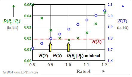
• It can also be seen from the graph that  $D(P_X \hspace{0.05cm}|| \hspace{0.05cm} P_Y) =0.0182$  bit  is not undercut by any  $λ$–value other than  $λ = 1$  (green crosses).
• Furthermore, one can see from this plot that a better entropy approximation is achieved with  $λ = 0.9$  than with  $λ = 1$  (blue circles):

$$H(Y) = 1.795\ {\rm bit} \hspace{0.15cm}\approx \hspace{0.15cm} H(X) = 1.793\ {\rm bit}\hspace{0.05cm}.$$

The second proposed solution is therefore wrong.

• With  $λ = 1$ , the  linear means  of the two random variables coincide:

$$m_X = m_Y= 1.$$

• With  $λ = 0.9$ the  quadratic means  agree:

$$m_X + \sigma_X^2 = m_Y + \sigma_Y^2= 1.8.$$

Whether this statement is relevant, we leave undecided.  Because:   Due to the steady increase of   $H(Y)$  with increasing  $λ$ , it is clear that for some  $λ$–value   $H(Y) = H(X)$  must indeed hold.