Difference between revisions of "Theory of Stochastic Signals/Digital Filters"
m (Rosa moved page Theory of Stochastic Signals/Digitale Filter to Theory of Stochastic Signals/Digital Filters) |
|||
| (7 intermediate revisions by 2 users not shown) | |||
| Line 1: | Line 1: | ||
{{Header | {{Header | ||
| − | |Untermenü= | + | |Untermenü=Filtering of Stochastic Signals |
|Vorherige Seite=Stochastische Systemtheorie | |Vorherige Seite=Stochastische Systemtheorie | ||
|Nächste Seite=Erzeugung vorgegebener AKF-Eigenschaften | |Nächste Seite=Erzeugung vorgegebener AKF-Eigenschaften | ||
}} | }} | ||
| − | == | + | ==General block diagram== |
<br> | <br> | ||
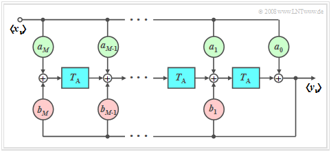
| − | + | Each signal $x(t)$ can be represented on a computer only by the sequence $〈x_ν〉$ of its samples, where $x_ν$ stands for $x(ν · T_{\rm A})$. | |
| − | [[File:P_ID552__Sto_T_5_2_S1_neu.png |right|frame| | + | [[File:P_ID552__Sto_T_5_2_S1_neu.png |right|frame| Block diagram of a digital filter]] |
| − | * | + | *The time interval $T_{\rm A}$ between two samples is thereby upper bounded by the [[Signal_Representation/Discrete-Time_Signal_Representation#Sampling_theorem|$\text{sampling theorem}$]]. |
| − | * | + | *To capture the influence of a linear filter with frequency response $H(f)$ on the discrete-time signal $〈x_ν〉$, it makes sense to also describe the filter in discrete time. |
| − | * | + | *On the right you can see the corresponding block diagram. |
| − | + | Thus, for the samples of the output signal applies: | |
:$$y_\nu = \sum\limits_{\mu = 0}^M {a_\mu } \cdot x_{\nu - \mu } + \sum\limits_{\mu = 1}^M {b_\mu } \cdot y_{\nu - \mu } .$$ | :$$y_\nu = \sum\limits_{\mu = 0}^M {a_\mu } \cdot x_{\nu - \mu } + \sum\limits_{\mu = 1}^M {b_\mu } \cdot y_{\nu - \mu } .$$ | ||
| + | |||
| + | The applet [[Applets:Digital_Filters|"Digital Filters"]] illustrates the subject matter of this chapter. | ||
<br clear=all> | <br clear=all> | ||
| − | + | The following should be noted here: | |
| − | * | + | *The first sum describes the dependence of the current output $y_ν$ on the current input $x_ν$ and on the $M$ previous input values $x_{ν–1}$, ... , $x_{ν–M}.$ |
| − | * | + | *The second sum characterizes the influence of $y_ν$ by the previous values $y_{ν–1}$, ... , $y_{ν–M}$ at the filter output. Thus, it indicates the recursive part of the filter. |
| − | * | + | *The integer parameter $M$ is called the »'''order'''« of the digital filter. |
| − | == | + | ==Non-recursive filter== |
<br> | <br> | ||
{{BlaueBox|TEXT= | {{BlaueBox|TEXT= | ||
| − | $\text{Definition:}$ | + | $\text{Definition:}$ If all feedback coefficients are $b_{\mu} = 0$, we speak of a »'''non-recursive filter'''«. Otherwise, the filter is "recursive".}} |
| − | + | Such a $M$–th order non-recursive filter has the following properties: | |
| − | [[File:P_ID553__Sto_T_5_2_S2_neu.png|right |frame| | + | [[File:P_ID553__Sto_T_5_2_S2_neu.png|right |frame| Non-recursive digital filter of order $M$]] |
| − | * | + | *The output value $y_ν$ depends only on the current and the $M$ previous input values: |
:$$y_\nu = \sum\limits_{\mu = 0}^M {a_\mu \cdot x_{\mu - \nu } } .$$ | :$$y_\nu = \sum\limits_{\mu = 0}^M {a_\mu \cdot x_{\mu - \nu } } .$$ | ||
| − | * | + | *The filter impulse response is obtained from this with $x(t) = δ(t)$: |
:$$h(t) = \sum\limits_{\mu = 0}^M {a_\mu \cdot \delta ( {t - \mu \cdot T_{\rm A} } )} .$$ | :$$h(t) = \sum\limits_{\mu = 0}^M {a_\mu \cdot \delta ( {t - \mu \cdot T_{\rm A} } )} .$$ | ||
| − | * | + | *The corresponding input signal in discrete-time notation is: $x_ν ≡0$ except for $x_0 =1$. |
| − | * | + | *By applying the shifting theorem, it follows for the filter frequency response: |
:$$H(f) = \sum\limits_{\mu = 0}^M {a_\mu \cdot {\rm{e}}^{ - {\rm{j}}\hspace{0.05cm} \cdot \hspace{0.05cm}2{\rm{\pi }}\hspace{0.05cm} \cdot \hspace{0.05cm}f \hspace{0.05cm} \cdot \hspace{0.05cm} \mu \hspace{0.05cm} \cdot \hspace{0.05cm} T_{\rm A} } } .$$ | :$$H(f) = \sum\limits_{\mu = 0}^M {a_\mu \cdot {\rm{e}}^{ - {\rm{j}}\hspace{0.05cm} \cdot \hspace{0.05cm}2{\rm{\pi }}\hspace{0.05cm} \cdot \hspace{0.05cm}f \hspace{0.05cm} \cdot \hspace{0.05cm} \mu \hspace{0.05cm} \cdot \hspace{0.05cm} T_{\rm A} } } .$$ | ||
{{GraueBox|TEXT= | {{GraueBox|TEXT= | ||
| − | $\text{ | + | $\text{Example 1:}$ A two-way channel, where |
| − | * | + | *the signal arrives on the main path unattenuated with respect to the input signal, but delayed by $2\ \rm µ s$, and |
| − | * | + | *is followed at a distance of $4\ \rm µ s$ – i.e. absolutely at time $t = 6\ \rm µ s$ – by an echo with half amplitude, |
| − | + | can be simulated by a non-recursive filter according to the above diagram, where the following parameter values are to be set: | |
:$$M = 3,\quad T_{\rm A} = 2\;{\rm{µ s} },\quad a_{\rm 0} = 0,\quad a_{\rm 1} = 1, \quad a_{\rm 2} = 0, \quad a_{\rm 3} = 0.5.$$}} | :$$M = 3,\quad T_{\rm A} = 2\;{\rm{µ s} },\quad a_{\rm 0} = 0,\quad a_{\rm 1} = 1, \quad a_{\rm 2} = 0, \quad a_{\rm 3} = 0.5.$$}} | ||
| − | == | + | ==Recursive filter== |
<br> | <br> | ||
{{BlaueBox|TEXT= | {{BlaueBox|TEXT= | ||
| − | $\text{Definition:}$ | + | $\text{Definition:}$ If all forward coefficients are $a_\nu \equiv 0$ with the exception of $a_0$, then a »'''(purely) recursive filter'''« is present.}} |
| − | [[File:P_ID554__Sto_T_5_2_S3_neu.png|right|frame| | + | [[File:P_ID554__Sto_T_5_2_S3_neu.png|right|frame| First-order recursive digital filter]] |
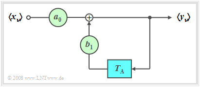
| − | + | In the following, we restrict ourselves to the special case $M = 1$ (block diagram corresponding to the figure). This filter has the following properties: | |
| − | * | + | *The output value $y_ν$ depends (indirectly) on an infinite number of input values: |
:$$y_\nu = \sum\limits_{\mu = 0}^\infty {a_0 \cdot {b_1} ^\mu \cdot x_{\nu - \mu } .}$$ | :$$y_\nu = \sum\limits_{\mu = 0}^\infty {a_0 \cdot {b_1} ^\mu \cdot x_{\nu - \mu } .}$$ | ||
| − | * | + | *This is shown by the following calculation: |
:$$y_\nu = a_0 \cdot x_\nu + b_1 \cdot y_{\nu - 1} = a_0 \cdot x_\nu + a_0 \cdot b_1 \cdot x_{\nu - 1} + {b_1} ^2 \cdot y_{\nu - 2}. $$ | :$$y_\nu = a_0 \cdot x_\nu + b_1 \cdot y_{\nu - 1} = a_0 \cdot x_\nu + a_0 \cdot b_1 \cdot x_{\nu - 1} + {b_1} ^2 \cdot y_{\nu - 2}. $$ | ||
| Line 64: | Line 66: | ||
{{BlaueBox|TEXT= | {{BlaueBox|TEXT= | ||
$\text{Definition:}$ | $\text{Definition:}$ | ||
| − | * | + | *The »'''discrete-time impulse response'''« $〈\hspace{0.05cm}h_\mu\hspace{0.05cm}〉$ is by definition the output sequence when a single »'''one'''« is present at the input at $t =0$. |
| − | * | + | *For a recursive filter, the discrete-time impulse response extends to infinity already with $M = 1$: |
:$$h(t)= \sum\limits_{\mu = 0}^\infty {a_0 \cdot {b_1} ^\mu \cdot \delta ( {t - \mu \cdot T_{\rm A} } )}\hspace{0.3cm} | :$$h(t)= \sum\limits_{\mu = 0}^\infty {a_0 \cdot {b_1} ^\mu \cdot \delta ( {t - \mu \cdot T_{\rm A} } )}\hspace{0.3cm} | ||
| − | \Rightarrow \hspace{0.3cm}〈\hspace{0.05cm}h_\mu\hspace{0.05cm}〉= 〈\hspace{0.05cm}a_0, \ a_0\cdot {b_1}, \ a_0\cdot {b_1}^2 \ \text{...} \hspace{0.05cm}〉.$$}} | + | \Rightarrow \hspace{0.3cm}〈\hspace{0.05cm}h_\mu\hspace{0.05cm}〉= 〈\hspace{0.05cm}a_0, \ a_0\cdot {b_1}, \ a_0\cdot {b_1}^2, \ a_0\cdot {b_1}^3, \ \text{...} \hspace{0.05cm}〉.$$}} |
| − | + | Further, it should be noted: | |
| − | * | + | *For stability reasons, $b_1 < 1$ must hold. |
| − | * | + | *If $b_1 = 1$, the impulse response $h(t)$ would extend to infinity and if $b_1 > 1$, $h(t)$ would even resonate to infinity. |
| − | * | + | *In such a first-order recursive filter, each individual Dirac delta line is smaller than the previous Dirac delta line by exactly the factor $b_1$: |
:$$h_{\mu} = h(\mu \cdot T_{\rm A}) = {b_1} \cdot h_{\mu -1}.$$ | :$$h_{\mu} = h(\mu \cdot T_{\rm A}) = {b_1} \cdot h_{\mu -1}.$$ | ||
| − | [[File:Sto_T_5_2_S3_version2.png |frame| | + | [[File:Sto_T_5_2_S3_version2.png |frame| Discrete-time impulse response <br>of a recursive digital filter | right]] |
{{GraueBox|TEXT= | {{GraueBox|TEXT= | ||
| − | $\text{ | + | $\text{Example 2:}$ The diagram on the right shows the discrete-time impulse response $〈\hspace{0.05cm}h_\mu\hspace{0.05cm}〉$ of a first-order recursive filter with the parameters $a_0 = 1$ and $b_1 = 0.6$. |
| − | * | + | *The progression is exponentially decreasing and extends to infinity–in–time. |
| − | * | + | *The ratio of the weights of two successive Dirac delta lines is $b_1 = 0.6$ in each case.}} |
| − | == | + | ==Exercises for the chapter== |
<br> | <br> | ||
| − | [[Aufgaben: | + | [[Aufgaben:Exercise_5.3:_1st_order_Digital_Filter|Exercise 5.3: 1st order Digital Filter]] |
| − | [[Aufgaben: | + | [[Aufgaben:Exercise_5.3Z:_Non-Recursive_Filter|Exercise 5.3Z: Non-Recursive Filter]] |
| − | [[Aufgaben: | + | [[Aufgaben:Exercise_5.4:_Sine_Wave_Generator|Exercise 5.4: Sine Wave Generator]] |
{{Display}} | {{Display}} | ||
Latest revision as of 14:39, 18 January 2023
Contents
General block diagram
Each signal $x(t)$ can be represented on a computer only by the sequence $〈x_ν〉$ of its samples, where $x_ν$ stands for $x(ν · T_{\rm A})$.
- The time interval $T_{\rm A}$ between two samples is thereby upper bounded by the $\text{sampling theorem}$.
- To capture the influence of a linear filter with frequency response $H(f)$ on the discrete-time signal $〈x_ν〉$, it makes sense to also describe the filter in discrete time.
- On the right you can see the corresponding block diagram.
Thus, for the samples of the output signal applies:
- $$y_\nu = \sum\limits_{\mu = 0}^M {a_\mu } \cdot x_{\nu - \mu } + \sum\limits_{\mu = 1}^M {b_\mu } \cdot y_{\nu - \mu } .$$
The applet "Digital Filters" illustrates the subject matter of this chapter.
The following should be noted here:
- The first sum describes the dependence of the current output $y_ν$ on the current input $x_ν$ and on the $M$ previous input values $x_{ν–1}$, ... , $x_{ν–M}.$
- The second sum characterizes the influence of $y_ν$ by the previous values $y_{ν–1}$, ... , $y_{ν–M}$ at the filter output. Thus, it indicates the recursive part of the filter.
- The integer parameter $M$ is called the »order« of the digital filter.
Non-recursive filter
$\text{Definition:}$ If all feedback coefficients are $b_{\mu} = 0$, we speak of a »non-recursive filter«. Otherwise, the filter is "recursive".
Such a $M$–th order non-recursive filter has the following properties:
- The output value $y_ν$ depends only on the current and the $M$ previous input values:
- $$y_\nu = \sum\limits_{\mu = 0}^M {a_\mu \cdot x_{\mu - \nu } } .$$
- The filter impulse response is obtained from this with $x(t) = δ(t)$:
- $$h(t) = \sum\limits_{\mu = 0}^M {a_\mu \cdot \delta ( {t - \mu \cdot T_{\rm A} } )} .$$
- The corresponding input signal in discrete-time notation is: $x_ν ≡0$ except for $x_0 =1$.
- By applying the shifting theorem, it follows for the filter frequency response:
- $$H(f) = \sum\limits_{\mu = 0}^M {a_\mu \cdot {\rm{e}}^{ - {\rm{j}}\hspace{0.05cm} \cdot \hspace{0.05cm}2{\rm{\pi }}\hspace{0.05cm} \cdot \hspace{0.05cm}f \hspace{0.05cm} \cdot \hspace{0.05cm} \mu \hspace{0.05cm} \cdot \hspace{0.05cm} T_{\rm A} } } .$$
$\text{Example 1:}$ A two-way channel, where
- the signal arrives on the main path unattenuated with respect to the input signal, but delayed by $2\ \rm µ s$, and
- is followed at a distance of $4\ \rm µ s$ – i.e. absolutely at time $t = 6\ \rm µ s$ – by an echo with half amplitude,
can be simulated by a non-recursive filter according to the above diagram, where the following parameter values are to be set:
- $$M = 3,\quad T_{\rm A} = 2\;{\rm{µ s} },\quad a_{\rm 0} = 0,\quad a_{\rm 1} = 1, \quad a_{\rm 2} = 0, \quad a_{\rm 3} = 0.5.$$
Recursive filter
$\text{Definition:}$ If all forward coefficients are $a_\nu \equiv 0$ with the exception of $a_0$, then a »(purely) recursive filter« is present.
In the following, we restrict ourselves to the special case $M = 1$ (block diagram corresponding to the figure). This filter has the following properties:
- The output value $y_ν$ depends (indirectly) on an infinite number of input values:
- $$y_\nu = \sum\limits_{\mu = 0}^\infty {a_0 \cdot {b_1} ^\mu \cdot x_{\nu - \mu } .}$$
- This is shown by the following calculation:
- $$y_\nu = a_0 \cdot x_\nu + b_1 \cdot y_{\nu - 1} = a_0 \cdot x_\nu + a_0 \cdot b_1 \cdot x_{\nu - 1} + {b_1} ^2 \cdot y_{\nu - 2}. $$
$\text{Definition:}$
- The »discrete-time impulse response« $〈\hspace{0.05cm}h_\mu\hspace{0.05cm}〉$ is by definition the output sequence when a single »one« is present at the input at $t =0$.
- For a recursive filter, the discrete-time impulse response extends to infinity already with $M = 1$:
- $$h(t)= \sum\limits_{\mu = 0}^\infty {a_0 \cdot {b_1} ^\mu \cdot \delta ( {t - \mu \cdot T_{\rm A} } )}\hspace{0.3cm} \Rightarrow \hspace{0.3cm}〈\hspace{0.05cm}h_\mu\hspace{0.05cm}〉= 〈\hspace{0.05cm}a_0, \ a_0\cdot {b_1}, \ a_0\cdot {b_1}^2, \ a_0\cdot {b_1}^3, \ \text{...} \hspace{0.05cm}〉.$$
Further, it should be noted:
- For stability reasons, $b_1 < 1$ must hold.
- If $b_1 = 1$, the impulse response $h(t)$ would extend to infinity and if $b_1 > 1$, $h(t)$ would even resonate to infinity.
- In such a first-order recursive filter, each individual Dirac delta line is smaller than the previous Dirac delta line by exactly the factor $b_1$:
- $$h_{\mu} = h(\mu \cdot T_{\rm A}) = {b_1} \cdot h_{\mu -1}.$$
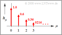
$\text{Example 2:}$ The diagram on the right shows the discrete-time impulse response $〈\hspace{0.05cm}h_\mu\hspace{0.05cm}〉$ of a first-order recursive filter with the parameters $a_0 = 1$ and $b_1 = 0.6$.
- The progression is exponentially decreasing and extends to infinity–in–time.
- The ratio of the weights of two successive Dirac delta lines is $b_1 = 0.6$ in each case.
Exercises for the chapter
Exercise 5.3: 1st order Digital Filter
Exercise 5.3Z: Non-Recursive Filter
Exercise 5.4: Sine Wave Generator


