Difference between revisions of "Theory of Stochastic Signals/Stochastic System Theory"
m (Text replacement - "„" to """) |
|||
| (17 intermediate revisions by 2 users not shown) | |||
| Line 1: | Line 1: | ||
{{Header | {{Header | ||
| − | |Untermenü= | + | |Untermenü=Filtering of Stochastic Signals |
|Vorherige Seite= Verallgemeinerung auf N-dimensionale Zufallsgrößen | |Vorherige Seite= Verallgemeinerung auf N-dimensionale Zufallsgrößen | ||
|Nächste Seite=Digitale Filter | |Nächste Seite=Digitale Filter | ||
}} | }} | ||
| − | == # | + | == # OVERVIEW OF THE FIFTH MAIN CHAPTER # == |
<br> | <br> | ||
| − | + | This chapter describes the influence of a filter on the »auto-correlation function« $\rm (ACF)$ and »the power-spectral density $\rm (PSD)$« of stochastic signals. | |
| − | + | In detail, this chapter covers: | |
| − | * | + | *the »calculation of ACF and PSD« at the filter output ("Stochastic System Theory"), |
| − | * | + | *the structure and representation of »digital filters« (non-recursive and recursive), |
| − | * | + | *the »dimensioning« of the filter coefficients for a given ACF, |
| − | * | + | *the meaning of the »matched filter« for the SNR maximization of communication systems, |
| − | * | + | *the properties of the »Wiener-Kolmogorow filter« for the signal reconstruction. |
| − | |||
| − | |||
| − | |||
| − | + | ==System model and problem definition== | |
| + | <br> | ||
| + | As in the book [[Linear_and_Time_Invariant_Systems|"Linear and Time Invariant Systems"]], we consider the setup sketched on the right, where the system characterized both | ||
| + | *by the impulse response $h(t)$ | ||
| + | *as well as by its frequency response $H(f)$ | ||
| − | |||
| − | |||
| + | is described unambiguously. The relationship between these descriptive quantities in the time and frequency domain is given by the [[Signal_Representation/Fourier_Transform_and_its_Inverse#Properties_of_aperiodic_signals|$\text{Fourier transformation}$]]. | ||
| + | [[File:EN_Sto_T_5_1_S1.png |right| 300px|frame|Filter influence on "spectrum" and <br>"power-spectral density"]] | ||
| − | + | <br>If we apply the signal $x(t)$ to the input and denote the output signal by $y(t)$, the classical system theory provides the following statements: | |
| − | <br> | + | *The output signal $y(t)$ results from the [[Signal_Representation/The_Convolution_Theorem_and_Operation|$\text{convolution}$]] between the input signal $x(t)$ and the impulse response $h(t)$. The following equation is equally valid for deterministic and stochastic signals: |
| − | |||
| − | |||
| − | |||
| − | |||
| − | |||
| − | |||
| − | |||
| − | |||
| − | |||
| − | * | ||
:$$y(t) = x(t) \ast h(t) = \int_{-\infty}^{+\infty} x(\tau)\cdot h ( t - \tau) \,\,{\rm d}\tau.$$ | :$$y(t) = x(t) \ast h(t) = \int_{-\infty}^{+\infty} x(\tau)\cdot h ( t - \tau) \,\,{\rm d}\tau.$$ | ||
| − | * | + | *For deterministic signals, one usually takes a roundabout route using the spectral functions. The spectrum $X(f)$ is the Fourier transform of $x(t)$. The multiplication with the frequency response $H(f)$ leads to the output spectrum $Y(f)$. From this, the signal $y(t)$ can be obtained by the Fourier inverse transformation. |
| − | * | + | *In the case of stochastic signals this procedure fails, because then the time functions $x(t)$ and $y(t)$ are not predictable for all times from $–∞$ to $+∞$ and thus, the corresponding amplitude spectra $X(f)$ and $Y(f)$ do not exist at all. In this case, we have to switch to the [[Theory_of_Stochastic_Signals/Power-Spectral_Density|$\text{power-spectral density}$]] defined in the last chapter. |
| − | |||
| − | == | + | ==Amplitude spectrum and power-spectral density== |
| + | <br> | ||
| + | We consider an ergodic random process $\{x(t)\}$, whose auto-correlation function $φ_x(τ)$ is assumed to be known. The power-spectral density ${\it Φ}_x(f)$ is then also uniquely determined via the Fourier transform and the following statements hold: | ||
| + | :[[File:P_ID467__Sto_T_5_1_S2_neu.png|right| |frame| For the ACF and PSD calculation of a random signal]] | ||
<br> | <br> | ||
| − | + | #The [[Theory_of_Stochastic_Signals/Power-Spectral_Density|$\text{power-spectral density}$]] ${\it Φ}_x(f)$ can be given – as well as the auto-correlation function $φ_x(τ)$ – for each individual pattern function of the stationary and ergodic random process $\{x(t)\}$, even if the specific course of $x(t)$ is explicitly unknown.<br><br> | |
| − | + | #The [[Signal_Representation/Fourier_Transform_and_its_Inverse#The_first_Fourier_integral|$\text{amplitude spectrum}$]] $X(f)$, on the other hand, is undefined because if the spectral function $X(f)$ is known, the entire time function $x(t)$ from $–∞$ to $+∞$ would also have to be known via the Fourier inverse transform, which clearly cannot be the case for a stochastic signal.<br><br> | |
| − | + | #If a time section of finite time duration $T_{\rm M}$ is known according to the sketch on the right, the Fourier transform can of course be applied to it again. | |
| − | |||
| − | |||
<br clear=all> | <br clear=all> | ||
{{BlaueBox|TEXT= | {{BlaueBox|TEXT= | ||
| − | $\text{ | + | $\text{Theorem:}$ The following relationship exists between the power-spectral density ${\it Φ}_x(f)$ of the infinite time random signal $x(t)$ and the amplitude spectrum $X_{\rm T}(f)$ of the finite time section $x_{\rm T}(t)$: |
:$${ {\it \Phi}_x(f)} = \lim_{T_{\rm M}\to\infty}\hspace{0.2cm} | :$${ {\it \Phi}_x(f)} = \lim_{T_{\rm M}\to\infty}\hspace{0.2cm} | ||
\frac{1}{ T_{\rm M} }\cdot \vert X_{\rm T}(f)\vert ^2.$$}} | \frac{1}{ T_{\rm M} }\cdot \vert X_{\rm T}(f)\vert ^2.$$}} | ||
| Line 64: | Line 55: | ||
{{BlaueBox|TEXT= | {{BlaueBox|TEXT= | ||
| − | $\text{ | + | $\text{Proof:}$ Previously, the |
| − | [[Theory_of_Stochastic_Signals/ | + | [[Theory_of_Stochastic_Signals/Auto-Correlation_Function_(ACF)|$\text{auto-correlation function}$]] of an ergodic process with the random signal $x(t)$ was given as follows: |
:$${ {\it \varphi}_x(\tau)} = \lim_{T_{\rm M}\to\infty}\hspace{0.2cm} | :$${ {\it \varphi}_x(\tau)} = \lim_{T_{\rm M}\to\infty}\hspace{0.2cm} | ||
\frac{1}{ T_{\rm M} }\cdot\int^{+T_{\rm M}/2}_{-T_{\rm | \frac{1}{ T_{\rm M} }\cdot\int^{+T_{\rm M}/2}_{-T_{\rm | ||
M}/2}x(t)\cdot x(t + \tau)\hspace{0.1cm} \rm d \it t.$$ | M}/2}x(t)\cdot x(t + \tau)\hspace{0.1cm} \rm d \it t.$$ | ||
| − | * | + | *It is permissible to replace the function $x(t)$, which is unbounded in time, by the function $x_{\rm T}(t)$, which is bounded on the time range $-T_{\rm M}/2$ to $+T_{\rm M}/2$. $x_{\rm T}(t)$ corresponds to the spectrum $X_{\rm T}(f)$, and by applying the [[Signal_Representation/Fourier_Transform_and_its_Inverse#The_first_Fourier_integral|$\text{first Fourier integral}$]] and the [[Signal_Representation/Fourier_Transform_Theorems#Shifting_Theorem|$\text{shifting theorem}$]]: |
:$${ {\it \varphi}_x(\tau)} = \lim_{T_{\rm M}\to\infty}\hspace{0.2cm} | :$${ {\it \varphi}_x(\tau)} = \lim_{T_{\rm M}\to\infty}\hspace{0.2cm} | ||
\frac{1}{ T_{\rm M} }\cdot \int^{+T_{\rm M}/2}_{-T_{\rm | \frac{1}{ T_{\rm M} }\cdot \int^{+T_{\rm M}/2}_{-T_{\rm | ||
| Line 75: | Line 66: | ||
T}(f)\cdot {\rm e}^{ {\rm j}2 \pi f ( t + \tau) } \hspace{0.1cm} | T}(f)\cdot {\rm e}^{ {\rm j}2 \pi f ( t + \tau) } \hspace{0.1cm} | ||
\rm d \it f \hspace{0.1cm} \rm d \it t.$$ | \rm d \it f \hspace{0.1cm} \rm d \it t.$$ | ||
| − | * | + | *After splitting the exponent and swapping the time and frequency integrals, we get: |
:$${ {\it \varphi}_x(\tau)} = \lim_{T_{\rm M}\to\infty}\hspace{0.2cm} | :$${ {\it \varphi}_x(\tau)} = \lim_{T_{\rm M}\to\infty}\hspace{0.2cm} | ||
\frac{1}{ T_{\rm M} }\cdot \int^{+\infty}_{-\infty}X_{\rm | \frac{1}{ T_{\rm M} }\cdot \int^{+\infty}_{-\infty}X_{\rm | ||
| Line 81: | Line 72: | ||
T}(t)\cdot {\rm e}^{ {\rm j}2 \pi f t } \hspace{0.1cm} \rm d \it | T}(t)\cdot {\rm e}^{ {\rm j}2 \pi f t } \hspace{0.1cm} \rm d \it | ||
t \right] \cdot {\rm e}^{ {\rm j}2 \pi f \tau} \hspace{0.1cm} \rm d \it f.$$ | t \right] \cdot {\rm e}^{ {\rm j}2 \pi f \tau} \hspace{0.1cm} \rm d \it f.$$ | ||
| − | * | + | *The inner integral describes the conjugate-complex spectrum ${X_{\rm T} }^{\star}(f)$. It further follows that: |
:$${ {\it \varphi}_x(\tau)} = \lim_{T_{\rm M}\to\infty}\hspace{0.2cm} | :$${ {\it \varphi}_x(\tau)} = \lim_{T_{\rm M}\to\infty}\hspace{0.2cm} | ||
\frac{1}{ T_{\rm M} }\cdot \int^{+\infty}_{-\infty}\vert X_{\rm | \frac{1}{ T_{\rm M} }\cdot \int^{+\infty}_{-\infty}\vert X_{\rm | ||
T}(f)\vert^2 \cdot {\rm e}^{ {\rm j}2 \pi f \tau} \hspace{0.1cm} \rm d | T}(f)\vert^2 \cdot {\rm e}^{ {\rm j}2 \pi f \tau} \hspace{0.1cm} \rm d | ||
\it f.$$ | \it f.$$ | ||
| − | * | + | *A comparison with the theorem from [https://en.wikipedia.org/wiki/Norbert_Wiener $\text{Wiener}$] and [https://en.wikipedia.org/wiki/Aleksandr_Khinchin $\text{Chintchin}$] which is always valid in ergodicity, |
:$${ {\it \varphi}_x(\tau)} = \int^{+\infty}_{-\infty}{\it \Phi}_x(f) | :$${ {\it \varphi}_x(\tau)} = \int^{+\infty}_{-\infty}{\it \Phi}_x(f) | ||
\cdot {\rm e}^{ {\rm j}2 \pi f \tau} \hspace{0.1cm} \rm d \it f ,$$ | \cdot {\rm e}^{ {\rm j}2 \pi f \tau} \hspace{0.1cm} \rm d \it f ,$$ | ||
| − | : | + | :shows the validity of the above relation: |
:$${ {\it \Phi}_x(f)} = \lim_{T_{\rm M}\to\infty}\hspace{0.2cm} | :$${ {\it \Phi}_x(f)} = \lim_{T_{\rm M}\to\infty}\hspace{0.2cm} | ||
\frac{1}{ T_{\rm M} }\cdot \vert X_{\rm T}(f)\vert^2.$$ | \frac{1}{ T_{\rm M} }\cdot \vert X_{\rm T}(f)\vert^2.$$ | ||
<div align="right">'''q.e.d.'''</div>}} | <div align="right">'''q.e.d.'''</div>}} | ||
| − | == | + | ==Power-spectral density of the filter output signal== |
<br> | <br> | ||
| − | + | Combining the statements made in the last two sections, we arrive at the following important result: | |
{{BlaueBox|TEXT= | {{BlaueBox|TEXT= | ||
| − | $\text{ | + | $\text{Theorem:}$ The power-spectral density $\rm (PSD)$ at the output of a linear time-invariant system with frequency response $H(f)$ is obtained as the product |
| + | *of the "input power-spectral density" ${\it Φ}_x(f)$ | ||
| + | *and the "power transfer function" $\vert H(f)\vert ^2$. | ||
:$${ {\it \Phi}_y(f)} = { {\it \Phi}_x(f)} \cdot \vert H(f)\vert ^2.$$}} | :$${ {\it \Phi}_y(f)} = { {\it \Phi}_x(f)} \cdot \vert H(f)\vert ^2.$$}} | ||
{{BlaueBox|TEXT= | {{BlaueBox|TEXT= | ||
| − | $\text{ | + | $\text{Proof:}$ Starting from the three relations already derived before: |
:$${ {\it \Phi}_x(f)} =\hspace{-0.1cm} \lim_{T_{\rm M}\to\infty}\hspace{0.01cm} | :$${ {\it \Phi}_x(f)} =\hspace{-0.1cm} \lim_{T_{\rm M}\to\infty}\hspace{0.01cm} | ||
| − | \frac{1}{ T_{\rm M} }\hspace{-0.05cm}\cdot\hspace{-0.05cm} \vert X_{\rm T}(f)\vert^2, | + | \frac{1}{ T_{\rm M} }\hspace{-0.05cm}\cdot\hspace{-0.05cm} \vert X_{\rm T}(f)\vert^2,$$ |
| − | { {\it \Phi}_y(f)} =\hspace{-0.1cm} \lim_{T_{\rm M}\to\infty}\hspace{0.01cm} | + | :$$ { {\it \Phi}_y(f)} =\hspace{-0.1cm} \lim_{T_{\rm M}\to\infty}\hspace{0.01cm} |
| − | \frac{1}{ T_{\rm M} }\hspace{-0.05cm}\cdot\hspace{-0.05cm}\vert Y_{\rm T}(f)\vert^2, | + | \frac{1}{ T_{\rm M} }\hspace{-0.05cm}\cdot\hspace{-0.05cm}\vert Y_{\rm T}(f)\vert^2, $$ |
| − | Y_{\rm T}(f) = X_{\rm T}(f) \hspace{-0.05cm}\cdot\hspace{-0.05cm} H(f).$$ | + | :$$Y_{\rm T}(f) = X_{\rm T}(f) \hspace{-0.05cm}\cdot\hspace{-0.05cm} H(f).$$ |
| − | + | ||
| + | Substituting these equations into each other, we get the above result. | ||
<div align="right">'''q.e.d.'''</div>}} | <div align="right">'''q.e.d.'''</div>}} | ||
| − | + | The following example illustrates the relationship with white noise. | |
| − | |||
{{GraueBox|TEXT= | {{GraueBox|TEXT= | ||
| − | $\text{ | + | $\text{Example 1:}$ |
| − | + | At the input of a Gaussian low-pass filter with the frequency response | |
:$$H(f) = {\rm e}^{- \pi \hspace{0.03cm}\cdot \hspace{0.03cm}(f/\Delta f)^2}$$ | :$$H(f) = {\rm e}^{- \pi \hspace{0.03cm}\cdot \hspace{0.03cm}(f/\Delta f)^2}$$ | ||
| − | + | [[File:P_ID468__Sto_T_5_1_S3_neu.png |right|frame| Filter influence in the frequency domain]] | |
| + | white noise $x(t)$ with noise power density ${ {\it \Phi}_x(f)} =N_0/2$ is present ⇒ two-sided representation. Then, the following holds for the power-spectral density of the output signal: | ||
:$${ {\it \Phi}_y(f)} = \frac {N_0}{2} \cdot {\rm e}^{- 2 \pi \hspace{0.03cm}\cdot \hspace{0.03cm}(f/\Delta | :$${ {\it \Phi}_y(f)} = \frac {N_0}{2} \cdot {\rm e}^{- 2 \pi \hspace{0.03cm}\cdot \hspace{0.03cm}(f/\Delta | ||
f)^2}.$$ | f)^2}.$$ | ||
| − | + | The diagram shows the signals and power-spectral densities at the filter input and output. | |
| − | + | Notes: | |
| − | # | + | #The signal $x(t)$ – strictly speaking – cannot be plotted at all, since it has an infinite power ⇒ integral over ${\it Φ}_x(f)$ from $-\infty$ to $+\infty$. |
| − | # | + | #The output signal $y(t)$ has a lower frequency than $x(t)$ and a finite power corresponding to the integral over ${\it Φ}_y(f)$. |
| − | # | + | #In one-sided representation, (only) for $f>0$ would hold: ${ {\it \Phi}_x(f)} =N_0$. The statements (1) and (2) would also apply here in the same way.}} |
| − | == | + | ==The auto-correlation function of the filter output signal== |
<br> | <br> | ||
| − | + | The calculated power-spectral density $\rm (PSD)$ can also be written as follows: | |
| − | :$${{\it \Phi}_y(f)} = {{\it \Phi}_x(f)} \cdot H(f) \cdot H^{\star}(f)$$ | + | :$${{\it \Phi}_y(f)} = {{\it \Phi}_x(f)} \cdot H(f) \cdot H^{\star}(f).$$ |
{{BlaueBox|TEXT= | {{BlaueBox|TEXT= | ||
| − | $\text{ | + | $\text{Theorem:}$ The corresponding auto-correlation function $\rm (ACF)$ is then obtained according to the [[Signal_Representation/Fourier_Transform_Laws|$\text{Fourier transform laws}$]] and by applying the [[Signal_Representation/The_Convolution_Theorem_and_Operation#Convolution_in_the_time_domain|$\text{convolution theorem}$]]: |
:$${ {\it \varphi}_y(\tau)} = { {\it \varphi}_x(\tau)} \ast h(\tau)\ast h(- | :$${ {\it \varphi}_y(\tau)} = { {\it \varphi}_x(\tau)} \ast h(\tau)\ast h(- | ||
\tau).$$}} | \tau).$$}} | ||
| − | + | In the transition from the spectral to the time domain, note: | |
| − | * | + | * The Fourier retransforms are to be inserted in each case, namely |
| − | :$${{\it \varphi}_y(\tau)} \circ\hspace{0.05cm}\!\!\!-\!\!\!-\!\!\!-\!\!\bullet\,{{\it \Phi}_y(f)}, \hspace{0.5cm}{{\it \varphi}_x(\tau)} \circ\hspace{0.05cm}\!\!\!-\!\!\!-\!\!\!-\!\!\!\bullet\,{{\it \Phi}_x(f)}, \hspace{0.5cm}{h(\tau)} \circ\hspace{0.05cm}\!\!\!-\!\!\!-\!\!\!-\!\!\bullet\,{H(f)}, \hspace{0.5cm}{h(-\tau)} \circ\hspace{0.05cm}\!\!\!-\!\!\!-\!\!\!-\!\!\!\bullet\,{H^{\star}(f)}$$ | + | :$${{\it \varphi}_y(\tau)} \circ\hspace{0.05cm}\!\!\!-\!\!\!-\!\!\!-\!\!\bullet\,{{\it \Phi}_y(f)}, \hspace{0.5cm}{{\it \varphi}_x(\tau)} \circ\hspace{0.05cm}\!\!\!-\!\!\!-\!\!\!-\!\!\!\bullet\,{{\it \Phi}_x(f)}, \hspace{0.5cm}{h(\tau)} \circ\hspace{0.05cm}\!\!\!-\!\!\!-\!\!\!-\!\!\bullet\,{H(f)}, \hspace{0.5cm}{h(-\tau)} \circ\hspace{0.05cm}\!\!\!-\!\!\!-\!\!\!-\!\!\!\bullet\,{H^{\star}(f)}.$$ |
| − | * | + | *Moreover, each multiplication becomes a convolution operation. |
| − | |||
{{GraueBox|TEXT= | {{GraueBox|TEXT= | ||
| − | $\text{ | + | $\text{Example 2:}$ |
| − | + | We consider again the same scenario as in [[Theory_of_Stochastic_Signals/Stochastic_System_Theory#Power-spectral_density_of_the_filter_output_signal| $\text{Example 1}$]], but this time in the time domain. It holds: | |
| − | * | + | [[File:P_ID591__Sto_T_5_1_S4_neu.png |right|frame| Filter influence in the time domain]] |
| − | + | *Two-sided white noise power density: ${ {\it \Phi}_x(f)} =N_0/2$, | |
| − | * | + | *Gaussian filter: $H(f) = {\rm e}^{- \pi \hspace{0.03cm}\cdot \hspace{0.03cm}(f/\Delta f)^2}\hspace{0.3cm}\Rightarrow \hspace{0.3cm} |
h(t) = \Delta f \cdot {\rm e}^{- \pi \hspace{0.03cm}\cdot \hspace{0.03cm}(\Delta f \hspace{0.03cm}\cdot \hspace{0.03cm}t)^2}.$ | h(t) = \Delta f \cdot {\rm e}^{- \pi \hspace{0.03cm}\cdot \hspace{0.03cm}(\Delta f \hspace{0.03cm}\cdot \hspace{0.03cm}t)^2}.$ | ||
| − | + | One can see from this diagram: | |
| − | # | + | #The ACF of the input signal is now a Dirac delta function with weight $N_0/2$. |
| − | # | + | #By convolution twice with the (here also Gaussian) impulse response $h(t)$ or $h(–t)$ one obtains the ACF $φ_y(τ)$ of the output signal. |
| − | # | + | #Thus, the ACF $φ_y(τ)$ of the output signal is also Gaussian. |
| − | # | + | #The ACF value at $τ = 0$ is identical to the area of the power-spectral density ${\it Φ}_y(f)$ and characterizes the signal power (variance) $σ_y^2$. |
| − | # | + | #In contrast, the area at $φ_y(τ)$ gives the PSD value: ${\it Φ}_y(f = \rm 0)=N_0/2$. }} |
| − | == | + | ==Cross-correlation function between input and output signal== |
<br> | <br> | ||
| − | [[File:EN_Sto_T_5_1_S5.png |frame| | + | [[File:EN_Sto_T_5_1_S5.png |frame| Calculating the cross-correlation function |right]] |
| − | + | We again consider a filter with the frequency response $H(f)$ and the impulse response $h(t)$. Further applies: | |
| − | + | ||
| − | + | #The stochastic input signal $x(t)$ is a sample function of the ergodic random process $\{x(t)\}$.<br><br> | |
| − | + | #The corresponding auto-correlation function $\rm (ACF)$ at the filter input is thus $φ_x(τ)$, while the power-spectral density $\rm (PSD)$ is denoted by ${\it Φ}_x(f)$. <br><br> | |
| + | #The corresponding descriptors of the ergodic random process $\{y(t)\}$ at the filter output are | ||
| + | |||
| + | ::*the random output signal $y(t)$, | ||
| + | ::*the auto-correlation function $φ_y(τ)$ | ||
| + | ::*and the conductance power-spectral density ${\it Φ}_y(f)$. | ||
<br clear=all> | <br clear=all> | ||
{{BlaueBox|TEXT= | {{BlaueBox|TEXT= | ||
| − | $\text{ | + | $\text{Theorem:}$ For the »'''cross-correlation function'''« $\rm (CCF)$ between the input and the output signal holds: |
:$${ {\it \varphi}_{xy}(\tau)} = h(\tau)\ast { {\it \varphi}_x(\tau)} .$$ | :$${ {\it \varphi}_{xy}(\tau)} = h(\tau)\ast { {\it \varphi}_x(\tau)} .$$ | ||
| − | + | Here, $h(τ)$ denotes the impulse response of the filter $($with the time variable $τ$ instead of $t)$ and ${ {\it \varphi}_{x}(\tau)}$ denotes the ACF of the input signal.}} | |
{{BlaueBox|TEXT= | {{BlaueBox|TEXT= | ||
| − | $\text{ | + | $\text{Proof:}$ In general, for the cross-correlation function between two signals $x(t)$ and $y(t)$: |
:$${ {\it \varphi}_{xy}(\tau)} = \lim_{T_{\rm M}\to\infty}\hspace{0.2cm}\frac{1}{ T_{\rm M} }\cdot\int^{+T_{\rm M}/2}_{-T_{\rm M}/2}x(t)\cdot y(t + \tau)\hspace{0.1cm} \rm d \it t.$$ | :$${ {\it \varphi}_{xy}(\tau)} = \lim_{T_{\rm M}\to\infty}\hspace{0.2cm}\frac{1}{ T_{\rm M} }\cdot\int^{+T_{\rm M}/2}_{-T_{\rm M}/2}x(t)\cdot y(t + \tau)\hspace{0.1cm} \rm d \it t.$$ | ||
| − | * | + | *With the generally valid relation $y(t) = h(t) \ast x(t)$ and the formal integration variable $θ$, we can also write for this: |
:$${ {\it \varphi}_{xy}(\tau)} = \lim_{T_{\rm M}\to\infty}\hspace{0.2cm}\frac{1}{ T_{\rm M} }\cdot\int^{+T_{\rm M}/2}_{-T_{\rm M}/2}x(t)\cdot \int^{+\infty}_{-\infty} h(\theta) \cdot x(t + \tau - \theta)\hspace{0.1cm}{\rm d}\theta\hspace{0.1cm}{\rm d} \it t.$$ | :$${ {\it \varphi}_{xy}(\tau)} = \lim_{T_{\rm M}\to\infty}\hspace{0.2cm}\frac{1}{ T_{\rm M} }\cdot\int^{+T_{\rm M}/2}_{-T_{\rm M}/2}x(t)\cdot \int^{+\infty}_{-\infty} h(\theta) \cdot x(t + \tau - \theta)\hspace{0.1cm}{\rm d}\theta\hspace{0.1cm}{\rm d} \it t.$$ | ||
| − | * | + | *By interchanging the two integrals and subtracting the limit into the integral, we obtain: |
:$${ {\it \varphi}_{xy}(\tau)} = \int^{+\infty}_{-\infty} | :$${ {\it \varphi}_{xy}(\tau)} = \int^{+\infty}_{-\infty} | ||
h(\theta) \cdot \left[ \lim_{T_{\rm M}\to\infty}\hspace{0.2cm} | h(\theta) \cdot \left[ \lim_{T_{\rm M}\to\infty}\hspace{0.2cm} | ||
| Line 190: | Line 188: | ||
M}/2}x(t)\cdot x(t + \tau - \theta)\hspace{0.1cm} | M}/2}x(t)\cdot x(t + \tau - \theta)\hspace{0.1cm} | ||
\hspace{0.1cm} {\rm d} t \right]{\rm d}\theta.$$ | \hspace{0.1cm} {\rm d} t \right]{\rm d}\theta.$$ | ||
| − | * | + | *The expression in the square brackets gives the ACF value at the input at time $τ - θ$: |
:$${ {\it \varphi}_{xy}(\tau)} = \int^{+\infty}_{-\infty}h(\theta) \cdot \varphi_x(\tau - \theta)\hspace{0.1cm}\hspace{0.1cm} {\rm d}\theta = h(\tau)\ast { {\it \varphi}_x(\tau)} .$$ | :$${ {\it \varphi}_{xy}(\tau)} = \int^{+\infty}_{-\infty}h(\theta) \cdot \varphi_x(\tau - \theta)\hspace{0.1cm}\hspace{0.1cm} {\rm d}\theta = h(\tau)\ast { {\it \varphi}_x(\tau)} .$$ | ||
| − | * | + | *However, the remaining integral describes the convolution operation in detailed notation. |
<div align="right">'''q.e.d.'''</div>}} | <div align="right">'''q.e.d.'''</div>}} | ||
{{BlaueBox|TEXT= | {{BlaueBox|TEXT= | ||
| − | $\text{ | + | $\text{Conclusion:}$ In the frequency domain, the corresponding equation is: |
:$${ {\it \Phi}_{xy}(f)} = H(f)\cdot{ {\it \Phi}_x(f)} \hspace{0.3cm} \Rightarrow \hspace{0.3cm} H(f) = \frac{ {\it \Phi}_{xy}(f)}{ {\it \Phi}_{x}(f)}.$$ | :$${ {\it \Phi}_{xy}(f)} = H(f)\cdot{ {\it \Phi}_x(f)} \hspace{0.3cm} \Rightarrow \hspace{0.3cm} H(f) = \frac{ {\it \Phi}_{xy}(f)}{ {\it \Phi}_{x}(f)}.$$ | ||
| − | + | This equation shows that the filter frequency response $H(f)$ from a measurement with stochastic excitation can be calculated completely – i.e., both magnitude and phase – if the following descriptive quantities are determined: | |
| − | * | + | *the statistical characteristics at the input, either the ACF $φ_x(τ)$ or the PSD ${\it Φ}_x(f)$, |
| − | * | + | *as well as the cross-correlation function $φ_{xy}(τ)$ or its Fourier transform ${\it Φ}_{xy}(f)$. }} |
| − | == | + | ==Exercises for the chapter== |
<br> | <br> | ||
| − | [[Aufgaben: | + | [[Aufgaben:Exercise_5.1:_Gaussian_ACF_and_Gaussian_Low-Pass|Exercise 5.1: Gaussian ACF and Gaussian Low-Pass]] |
| − | [[Aufgaben: | + | [[Aufgaben:Exercise_5.1Z:_Cosine_Square_Noise_Limitation|Exercise 5.1Z: Cosine Square Noise Limitation]] |
| − | [[Aufgaben:Aufgabe_5.2:_Bestimmung_des_Frequenzgangs| | + | [[Aufgaben:Aufgabe_5.2:_Bestimmung_des_Frequenzgangs|Exercise 5.2: Determination of the Frequency Response]] |
| − | [[Aufgaben: | + | [[Aufgaben:Exercise_5.2Z:_Two-Way_Channel|Exercise 5.2Z: Two-Way Channel]] |
{{Display}} | {{Display}} | ||
Latest revision as of 11:17, 22 December 2022
Contents
- 1 # OVERVIEW OF THE FIFTH MAIN CHAPTER #
- 2 System model and problem definition
- 3 Amplitude spectrum and power-spectral density
- 4 Power-spectral density of the filter output signal
- 5 The auto-correlation function of the filter output signal
- 6 Cross-correlation function between input and output signal
- 7 Exercises for the chapter
# OVERVIEW OF THE FIFTH MAIN CHAPTER #
This chapter describes the influence of a filter on the »auto-correlation function« $\rm (ACF)$ and »the power-spectral density $\rm (PSD)$« of stochastic signals.
In detail, this chapter covers:
- the »calculation of ACF and PSD« at the filter output ("Stochastic System Theory"),
- the structure and representation of »digital filters« (non-recursive and recursive),
- the »dimensioning« of the filter coefficients for a given ACF,
- the meaning of the »matched filter« for the SNR maximization of communication systems,
- the properties of the »Wiener-Kolmogorow filter« for the signal reconstruction.
System model and problem definition
As in the book "Linear and Time Invariant Systems", we consider the setup sketched on the right, where the system characterized both
- by the impulse response $h(t)$
- as well as by its frequency response $H(f)$
is described unambiguously. The relationship between these descriptive quantities in the time and frequency domain is given by the $\text{Fourier transformation}$.

"power-spectral density"
If we apply the signal $x(t)$ to the input and denote the output signal by $y(t)$, the classical system theory provides the following statements:
- The output signal $y(t)$ results from the $\text{convolution}$ between the input signal $x(t)$ and the impulse response $h(t)$. The following equation is equally valid for deterministic and stochastic signals:
- $$y(t) = x(t) \ast h(t) = \int_{-\infty}^{+\infty} x(\tau)\cdot h ( t - \tau) \,\,{\rm d}\tau.$$
- For deterministic signals, one usually takes a roundabout route using the spectral functions. The spectrum $X(f)$ is the Fourier transform of $x(t)$. The multiplication with the frequency response $H(f)$ leads to the output spectrum $Y(f)$. From this, the signal $y(t)$ can be obtained by the Fourier inverse transformation.
- In the case of stochastic signals this procedure fails, because then the time functions $x(t)$ and $y(t)$ are not predictable for all times from $–∞$ to $+∞$ and thus, the corresponding amplitude spectra $X(f)$ and $Y(f)$ do not exist at all. In this case, we have to switch to the $\text{power-spectral density}$ defined in the last chapter.
Amplitude spectrum and power-spectral density
We consider an ergodic random process $\{x(t)\}$, whose auto-correlation function $φ_x(τ)$ is assumed to be known. The power-spectral density ${\it Φ}_x(f)$ is then also uniquely determined via the Fourier transform and the following statements hold:
 For the ACF and PSD calculation of a random signal

- The $\text{power-spectral density}$ ${\it Φ}_x(f)$ can be given – as well as the auto-correlation function $φ_x(τ)$ – for each individual pattern function of the stationary and ergodic random process $\{x(t)\}$, even if the specific course of $x(t)$ is explicitly unknown.
- The $\text{amplitude spectrum}$ $X(f)$, on the other hand, is undefined because if the spectral function $X(f)$ is known, the entire time function $x(t)$ from $–∞$ to $+∞$ would also have to be known via the Fourier inverse transform, which clearly cannot be the case for a stochastic signal.
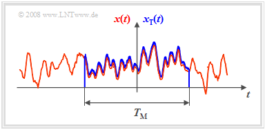
- If a time section of finite time duration $T_{\rm M}$ is known according to the sketch on the right, the Fourier transform can of course be applied to it again.
$\text{Theorem:}$ The following relationship exists between the power-spectral density ${\it Φ}_x(f)$ of the infinite time random signal $x(t)$ and the amplitude spectrum $X_{\rm T}(f)$ of the finite time section $x_{\rm T}(t)$:
- $${ {\it \Phi}_x(f)} = \lim_{T_{\rm M}\to\infty}\hspace{0.2cm} \frac{1}{ T_{\rm M} }\cdot \vert X_{\rm T}(f)\vert ^2.$$
$\text{Proof:}$ Previously, the $\text{auto-correlation function}$ of an ergodic process with the random signal $x(t)$ was given as follows:
- $${ {\it \varphi}_x(\tau)} = \lim_{T_{\rm M}\to\infty}\hspace{0.2cm} \frac{1}{ T_{\rm M} }\cdot\int^{+T_{\rm M}/2}_{-T_{\rm M}/2}x(t)\cdot x(t + \tau)\hspace{0.1cm} \rm d \it t.$$
- It is permissible to replace the function $x(t)$, which is unbounded in time, by the function $x_{\rm T}(t)$, which is bounded on the time range $-T_{\rm M}/2$ to $+T_{\rm M}/2$. $x_{\rm T}(t)$ corresponds to the spectrum $X_{\rm T}(f)$, and by applying the $\text{first Fourier integral}$ and the $\text{shifting theorem}$:
- $${ {\it \varphi}_x(\tau)} = \lim_{T_{\rm M}\to\infty}\hspace{0.2cm} \frac{1}{ T_{\rm M} }\cdot \int^{+T_{\rm M}/2}_{-T_{\rm M}/2}x_{\rm T}(t)\cdot \int^{+\infty}_{-\infty}X_{\rm T}(f)\cdot {\rm e}^{ {\rm j}2 \pi f ( t + \tau) } \hspace{0.1cm} \rm d \it f \hspace{0.1cm} \rm d \it t.$$
- After splitting the exponent and swapping the time and frequency integrals, we get:
- $${ {\it \varphi}_x(\tau)} = \lim_{T_{\rm M}\to\infty}\hspace{0.2cm} \frac{1}{ T_{\rm M} }\cdot \int^{+\infty}_{-\infty}X_{\rm T}(f)\cdot \left[ \int^{+T_{\rm M}/2}_{-T_{\rm M}/2}x_{\rm T}(t)\cdot {\rm e}^{ {\rm j}2 \pi f t } \hspace{0.1cm} \rm d \it t \right] \cdot {\rm e}^{ {\rm j}2 \pi f \tau} \hspace{0.1cm} \rm d \it f.$$
- The inner integral describes the conjugate-complex spectrum ${X_{\rm T} }^{\star}(f)$. It further follows that:
- $${ {\it \varphi}_x(\tau)} = \lim_{T_{\rm M}\to\infty}\hspace{0.2cm} \frac{1}{ T_{\rm M} }\cdot \int^{+\infty}_{-\infty}\vert X_{\rm T}(f)\vert^2 \cdot {\rm e}^{ {\rm j}2 \pi f \tau} \hspace{0.1cm} \rm d \it f.$$
- A comparison with the theorem from $\text{Wiener}$ and $\text{Chintchin}$ which is always valid in ergodicity,
- $${ {\it \varphi}_x(\tau)} = \int^{+\infty}_{-\infty}{\it \Phi}_x(f) \cdot {\rm e}^{ {\rm j}2 \pi f \tau} \hspace{0.1cm} \rm d \it f ,$$
- shows the validity of the above relation:
- $${ {\it \Phi}_x(f)} = \lim_{T_{\rm M}\to\infty}\hspace{0.2cm} \frac{1}{ T_{\rm M} }\cdot \vert X_{\rm T}(f)\vert^2.$$
Power-spectral density of the filter output signal
Combining the statements made in the last two sections, we arrive at the following important result:
$\text{Theorem:}$ The power-spectral density $\rm (PSD)$ at the output of a linear time-invariant system with frequency response $H(f)$ is obtained as the product
- of the "input power-spectral density" ${\it Φ}_x(f)$
- and the "power transfer function" $\vert H(f)\vert ^2$.
- $${ {\it \Phi}_y(f)} = { {\it \Phi}_x(f)} \cdot \vert H(f)\vert ^2.$$
$\text{Proof:}$ Starting from the three relations already derived before:
- $${ {\it \Phi}_x(f)} =\hspace{-0.1cm} \lim_{T_{\rm M}\to\infty}\hspace{0.01cm} \frac{1}{ T_{\rm M} }\hspace{-0.05cm}\cdot\hspace{-0.05cm} \vert X_{\rm T}(f)\vert^2,$$
- $$ { {\it \Phi}_y(f)} =\hspace{-0.1cm} \lim_{T_{\rm M}\to\infty}\hspace{0.01cm} \frac{1}{ T_{\rm M} }\hspace{-0.05cm}\cdot\hspace{-0.05cm}\vert Y_{\rm T}(f)\vert^2, $$
- $$Y_{\rm T}(f) = X_{\rm T}(f) \hspace{-0.05cm}\cdot\hspace{-0.05cm} H(f).$$
Substituting these equations into each other, we get the above result.
The following example illustrates the relationship with white noise.
$\text{Example 1:}$ At the input of a Gaussian low-pass filter with the frequency response
- $$H(f) = {\rm e}^{- \pi \hspace{0.03cm}\cdot \hspace{0.03cm}(f/\Delta f)^2}$$

white noise $x(t)$ with noise power density ${ {\it \Phi}_x(f)} =N_0/2$ is present ⇒ two-sided representation. Then, the following holds for the power-spectral density of the output signal:
- $${ {\it \Phi}_y(f)} = \frac {N_0}{2} \cdot {\rm e}^{- 2 \pi \hspace{0.03cm}\cdot \hspace{0.03cm}(f/\Delta f)^2}.$$
The diagram shows the signals and power-spectral densities at the filter input and output.
Notes:
- The signal $x(t)$ – strictly speaking – cannot be plotted at all, since it has an infinite power ⇒ integral over ${\it Φ}_x(f)$ from $-\infty$ to $+\infty$.
- The output signal $y(t)$ has a lower frequency than $x(t)$ and a finite power corresponding to the integral over ${\it Φ}_y(f)$.
- In one-sided representation, (only) for $f>0$ would hold: ${ {\it \Phi}_x(f)} =N_0$. The statements (1) and (2) would also apply here in the same way.
The auto-correlation function of the filter output signal
The calculated power-spectral density $\rm (PSD)$ can also be written as follows:
- $${{\it \Phi}_y(f)} = {{\it \Phi}_x(f)} \cdot H(f) \cdot H^{\star}(f).$$
$\text{Theorem:}$ The corresponding auto-correlation function $\rm (ACF)$ is then obtained according to the $\text{Fourier transform laws}$ and by applying the $\text{convolution theorem}$:
- $${ {\it \varphi}_y(\tau)} = { {\it \varphi}_x(\tau)} \ast h(\tau)\ast h(- \tau).$$
In the transition from the spectral to the time domain, note:
- The Fourier retransforms are to be inserted in each case, namely
- $${{\it \varphi}_y(\tau)} \circ\hspace{0.05cm}\!\!\!-\!\!\!-\!\!\!-\!\!\bullet\,{{\it \Phi}_y(f)}, \hspace{0.5cm}{{\it \varphi}_x(\tau)} \circ\hspace{0.05cm}\!\!\!-\!\!\!-\!\!\!-\!\!\!\bullet\,{{\it \Phi}_x(f)}, \hspace{0.5cm}{h(\tau)} \circ\hspace{0.05cm}\!\!\!-\!\!\!-\!\!\!-\!\!\bullet\,{H(f)}, \hspace{0.5cm}{h(-\tau)} \circ\hspace{0.05cm}\!\!\!-\!\!\!-\!\!\!-\!\!\!\bullet\,{H^{\star}(f)}.$$
- Moreover, each multiplication becomes a convolution operation.
$\text{Example 2:}$ We consider again the same scenario as in $\text{Example 1}$, but this time in the time domain. It holds:

- Two-sided white noise power density: ${ {\it \Phi}_x(f)} =N_0/2$,
- Gaussian filter: $H(f) = {\rm e}^{- \pi \hspace{0.03cm}\cdot \hspace{0.03cm}(f/\Delta f)^2}\hspace{0.3cm}\Rightarrow \hspace{0.3cm} h(t) = \Delta f \cdot {\rm e}^{- \pi \hspace{0.03cm}\cdot \hspace{0.03cm}(\Delta f \hspace{0.03cm}\cdot \hspace{0.03cm}t)^2}.$
One can see from this diagram:
- The ACF of the input signal is now a Dirac delta function with weight $N_0/2$.
- By convolution twice with the (here also Gaussian) impulse response $h(t)$ or $h(–t)$ one obtains the ACF $φ_y(τ)$ of the output signal.
- Thus, the ACF $φ_y(τ)$ of the output signal is also Gaussian.
- The ACF value at $τ = 0$ is identical to the area of the power-spectral density ${\it Φ}_y(f)$ and characterizes the signal power (variance) $σ_y^2$.
- In contrast, the area at $φ_y(τ)$ gives the PSD value: ${\it Φ}_y(f = \rm 0)=N_0/2$.
Cross-correlation function between input and output signal

We again consider a filter with the frequency response $H(f)$ and the impulse response $h(t)$. Further applies:
- The stochastic input signal $x(t)$ is a sample function of the ergodic random process $\{x(t)\}$.
- The corresponding auto-correlation function $\rm (ACF)$ at the filter input is thus $φ_x(τ)$, while the power-spectral density $\rm (PSD)$ is denoted by ${\it Φ}_x(f)$.
- The corresponding descriptors of the ergodic random process $\{y(t)\}$ at the filter output are
- the random output signal $y(t)$,
- the auto-correlation function $φ_y(τ)$
- and the conductance power-spectral density ${\it Φ}_y(f)$.
$\text{Theorem:}$ For the »cross-correlation function« $\rm (CCF)$ between the input and the output signal holds:
- $${ {\it \varphi}_{xy}(\tau)} = h(\tau)\ast { {\it \varphi}_x(\tau)} .$$
Here, $h(τ)$ denotes the impulse response of the filter $($with the time variable $τ$ instead of $t)$ and ${ {\it \varphi}_{x}(\tau)}$ denotes the ACF of the input signal.
$\text{Proof:}$ In general, for the cross-correlation function between two signals $x(t)$ and $y(t)$:
- $${ {\it \varphi}_{xy}(\tau)} = \lim_{T_{\rm M}\to\infty}\hspace{0.2cm}\frac{1}{ T_{\rm M} }\cdot\int^{+T_{\rm M}/2}_{-T_{\rm M}/2}x(t)\cdot y(t + \tau)\hspace{0.1cm} \rm d \it t.$$
- With the generally valid relation $y(t) = h(t) \ast x(t)$ and the formal integration variable $θ$, we can also write for this:
- $${ {\it \varphi}_{xy}(\tau)} = \lim_{T_{\rm M}\to\infty}\hspace{0.2cm}\frac{1}{ T_{\rm M} }\cdot\int^{+T_{\rm M}/2}_{-T_{\rm M}/2}x(t)\cdot \int^{+\infty}_{-\infty} h(\theta) \cdot x(t + \tau - \theta)\hspace{0.1cm}{\rm d}\theta\hspace{0.1cm}{\rm d} \it t.$$
- By interchanging the two integrals and subtracting the limit into the integral, we obtain:
- $${ {\it \varphi}_{xy}(\tau)} = \int^{+\infty}_{-\infty} h(\theta) \cdot \left[ \lim_{T_{\rm M}\to\infty}\hspace{0.2cm} \frac{1}{ T_{\rm M} } \cdot\int^{+T_{\rm M}/2}_{-T_{\rm M}/2}x(t)\cdot x(t + \tau - \theta)\hspace{0.1cm} \hspace{0.1cm} {\rm d} t \right]{\rm d}\theta.$$
- The expression in the square brackets gives the ACF value at the input at time $τ - θ$:
- $${ {\it \varphi}_{xy}(\tau)} = \int^{+\infty}_{-\infty}h(\theta) \cdot \varphi_x(\tau - \theta)\hspace{0.1cm}\hspace{0.1cm} {\rm d}\theta = h(\tau)\ast { {\it \varphi}_x(\tau)} .$$
- However, the remaining integral describes the convolution operation in detailed notation.
$\text{Conclusion:}$ In the frequency domain, the corresponding equation is:
- $${ {\it \Phi}_{xy}(f)} = H(f)\cdot{ {\it \Phi}_x(f)} \hspace{0.3cm} \Rightarrow \hspace{0.3cm} H(f) = \frac{ {\it \Phi}_{xy}(f)}{ {\it \Phi}_{x}(f)}.$$
This equation shows that the filter frequency response $H(f)$ from a measurement with stochastic excitation can be calculated completely – i.e., both magnitude and phase – if the following descriptive quantities are determined:
- the statistical characteristics at the input, either the ACF $φ_x(τ)$ or the PSD ${\it Φ}_x(f)$,
- as well as the cross-correlation function $φ_{xy}(τ)$ or its Fourier transform ${\it Φ}_{xy}(f)$.
Exercises for the chapter
Exercise 5.1: Gaussian ACF and Gaussian Low-Pass
Exercise 5.1Z: Cosine Square Noise Limitation
Exercise 5.2: Determination of the Frequency Response
Exercise 5.2Z: Two-Way Channel