Difference between revisions of "Mobile Communications/General Description of Time Variant Systems"
| Line 61: | Line 61: | ||
== Time invariant vs. time variant channels == | == Time invariant vs. time variant channels == | ||
<br> | <br> | ||
| − | The graphic is intended to illustrate the difference between a time invariant channel $\rm (LTI)$ and a time variant channel $\rm (LTV)$ .<br> | + | The graphic is intended to illustrate the difference between a linear time–invariant channel $\rm (LTI)$ and a linear time–variant channel $\rm (LTV)$ .<br> |
[[File:EN_Mob_T_2_1_S2.png|right|frame|Time invariant and time variant channel|class=fit]] | [[File:EN_Mob_T_2_1_S2.png|right|frame|Time invariant and time variant channel|class=fit]] | ||
| Line 84: | Line 84: | ||
$\text{Conclusion:}$ With a '''time-variant channel''' you cannot specify neither a one-parameter impulse response $h(t)$ nor a transfer function $H(f)$ .}}<br> | $\text{Conclusion:}$ With a '''time-variant channel''' you cannot specify neither a one-parameter impulse response $h(t)$ nor a transfer function $H(f)$ .}}<br> | ||
| − | <i>Note:</i> The learning video [[Eigenschaften_des_Übertragungskanals_(Lernvideo)|Properties of the transmission channel]] describes the differences between LTI and LTV systems.<br> | + | <i>Note:</i> The learning video [[Eigenschaften_des_Übertragungskanals_(Lernvideo)|Properties of the transmission channel]] (in German language) describes the differences between LTI and LTV systems.<br> |
== Two-dimensional impulse response== | == Two-dimensional impulse response== | ||
Revision as of 18:54, 10 December 2020
Contents
# SYNOPSIS OF THE SECOND MAIN CHAPTER #
After the time variance, the term Frequency Selectivity is now introduced and illustrated with examples, a channel property which is also of great importance for mobile communications. As in the entire book, the description is given in the equivalent low-pass range.
It is covered in detail:
- the difference between time invariant and time variant systems,
- the time variant impulse response as an important descriptive function of time variant systems,
- multi-way reception as the cause of frequency-selective behaviour,
- a detailed derivation and interpretation of the GWSSUS channel model,
- the characteristics of the GWSSUS model: coherence bandwidth, correlation duration, etc.
Transfer function and impulse response
The description parameters of a communication system have already been described in the chapters
of the book "Linear Time Variant Systems".
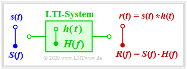
The most important results are briefly explained again here. We assume a linear and time invariant system ⇒ LTI system with the signal $s(t)$ at the input and the output signal $r(t)$. For the sake of simplicity, let $s(t)$ and $r(t)$ be real. Then the following applies:
- The system can be completely characterized by the transfer function $H(f)$ which is also referred to as the frequency response. By definition :$$H(f) = R(f)/S(f).$$
- Similarly, the system is defined by the impulse response $h(t)$ , which is the inverse Fourier transformation of $H(f)$. The output signal results from the convolution:
- \[r(t) = s(t) \star h(t) \hspace{0.4cm} {\rm with} \hspace{0.4cm} h(t) \hspace{0.2cm} \circ\!\!-\!\!\!-\!\!\!-\!\!\bullet \hspace{0.2cm} H(f) \hspace{0.05cm}.\]
$\text{Definitions:}$
The following input signals are suitable for detecting the linear distortions caused by $H(f)$ or $h(t)$
- $$s(t) = \delta(t) \hspace{0.3cm}\Rightarrow \hspace{0.3cm} r(t) = \delta(t) \star h(t)= h(t)\hspace{0.3cm}\Rightarrow \hspace{0.3cm} \text{impulse response,}$$
- $$s(t) = \gamma(t) \hspace{0.3cm}\Rightarrow \hspace{0.3cm} r(t) = \gamma(t) \star h(t)\hspace{1.5cm}\Rightarrow \hspace{0.3cm} \text{step response,}$$
- $$s(t) = p_\delta(t) \hspace{0.25cm}\Rightarrow \hspace{0.3cm} r(t) = p_\delta(t) \star h(t)\hspace{1.3cm}\Rightarrow \hspace{0.3cm} \text{impulse response train.}$$
- On the other hand, a DC signal $s(t) = A$ is not suitable to make the frequency dependence of the LTI system visible: With a low-pass system the output signal would then be always constant, independent of $H(f)$: $r(t) = A \cdot H(f= 0)$.
- On the next page we consider a Dirac impulse train $p_\delta(t)$ as an input signal $s(t)$: Hereby the similarities and differences between time-invariant and time-variant systems can be shown clearly.
- Note: The properties of $H(f)$ and $h(t)$ are covered in detail in the learning video Some remarks on the transfer function (in German language).
Time invariant vs. time variant channels
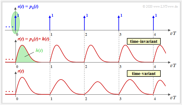
The graphic is intended to illustrate the difference between a linear time–invariant channel $\rm (LTI)$ and a linear time–variant channel $\rm (LTV)$ .
One can see from this illustration:
- The transmitted signal $s(t)$ is a Dirac impulse train $p_\delta(t)$, i.e. an infinite sequence of Dirac impulses in equidistant intervals $T$, all with the weight $1$ (see upper graph):
- \[s(t) = p_{\rm \delta} (t) = \sum_{n = -\infty}^{+\infty} {\rm \delta} (t - n \cdot T) \hspace{0.05cm}.\]
- The Dirac impulse at $t = 0$ is marked in green. The signal at the channel output is equal to $r(t) = h(t)$ , with $s(t) = {\rm \delta}(t)$ , also indicated in green. As a condition, it is assumed that the extension of the impulse response $h(t)$ is smaller than $T$.
.
- The entire received signal after the LTI channel, according to the middle graph, can then be written as:
- \[r(t) = p_{\rm \delta} (t) \star h(t) = \sum_{n = -\infty}^{+\infty} h (t - n \cdot T) \hspace{0.05cm}.\]
- For a time-variant channel (lower graph) this equation is not applicable. In each time interval, a (slightly) different signal shape is obtained.
$\text{Conclusion:}$ With a time-variant channel you cannot specify neither a one-parameter impulse response $h(t)$ nor a transfer function $H(f)$ .
Note: The learning video Properties of the transmission channel (in German language) describes the differences between LTI and LTV systems.
Two-dimensional impulse response
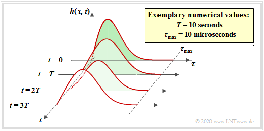
To identify a time-variant impulse response, a second parameter is used and the impulse response is preferably mapped in a three-dimensional coordinate system.
The condition for this is that the channel is still linear; one speaks then of a $\rm LTV System$ ("linear time-variant").
The following relations apply:
- \[\text{LTI:}\hspace{0.5cm} r(t) = \int_{-\infty}^{+\infty} h(\tau) \cdot s(t-\tau) \hspace{0.15cm}{\rm d}\tau \hspace{0.05cm},\]
- \[\text{LTV:}\hspace{0.5cm} r(t) \hspace{-0.1cm} = \hspace{-0.1cm} \int_{-\infty}^{+\infty} h(\tau, \hspace{0.1cm}t) \cdot s(t-\tau) \hspace{0.15cm}{\rm d}\tau \hspace{0.05cm}.\]
Regarding the last equation and the above graph, it should be noted
- The parameter $\tau$ specifies the Delay time to denote the time dispersion. By writing out the convolution operation, it was possible to make $\tau$ also the parameter of the LTI–impulse response. On the last pages we spoke about $h(t)$ .
- The second parameter of the impulse response or the second axis marks the absolute time $t$, which is used, among other things, to describe the time variance. At different times $t$ the impulse response $h(\tau, \hspace{0.05cm}t)$ has a different form.
- A peculiarity of the 2D representation is that the $t$–axis is always plotted time-discretely $($at multiples of $T)$ while the $\tau$–axis can be continuous in time as in the example shown. However, in mobile communications, a time-discrete $h(\tau, \hspace{0.05cm}t_0)$ with respect to $\tau$ is assumed $($„echoes”$)$.
- The LTV–equation is only applicable if the time change of the channel is slow in comparison to the maximum delay $\tau_{\rm max}$ $($marked in the figure by the parameter $T$ $)$. In mobile communications this condition ⇒ $\tau_{\rm max} < T$ is almost always fulfilled.
- Selecting whether to apply the first Fourier integral to the parameter $\tau$ or $t$ leads to different spectral functions. In the Exercise 2.1Z for example, the time variant 2D–Transfer function is considered:
- \[H(f,\hspace{0.05cm} t) \hspace{0.2cm} \bullet\!\!-\!\!\!-\!\!\!-\!\!\circ \hspace{0.2cm} h(\tau,\hspace{0.05cm}t) \hspace{0.05cm}.\]
Exercises to the chapter
Exercise 2.1: Two-Dimensional Impulse Response
Exercise 2.1Z: 2D-Frequency and 2D-Time Representations


