Probability Density of Rayleigh Fading

A very general description of the mobile communication channel

To simplify the notation, the addition "TP" (Tiefpass ⇒ low pass) is omitted in the following. Thus the real signal $s(t) = 1$ is present at the input of the mobile radio channel and the output signal $r(t)$ is complex-valued. Additional noise processes are excluded.

The radio signal $s(t)$ can reach the receiver via a large number of paths, whereby the individual signal components are attenuated in different ways and delayed for different lengths. In general, it is possible to express the received signal (in the equivalent low pass range) without taking thermal noise into account as it follows:

\[r(t)= \sum_{k=1}^{K} \alpha_{k}(t) \cdot {\rm e}^{\hspace{0.05cm}{\rm j}\hspace{0.02cm}\cdot \hspace{0.02cm} \phi_{k}(t)} \cdot s(t - \tau_{k}) \hspace{0.05cm}.\]

The following designations are used here:

The time dependent attenuation factor on the $k$–th path is $\alpha_k(t)$.

The time dependent phase progression on the $k$–th path is $\phi_k(t)$.

The time dependent runtime on the $k$–th path is $\tau_k(t)$.

The number $K$ of (at least slightly) different paths is usually very large and unsuitable for direct modeling.

The model can be simplified considerably by combining paths with approximately equal delays.
So you only distinguish between $M$ main paths, which are characterized by large differences in distance and thus noticeable differences in delay:

\[r(t)= \sum_{m=1}^{M} \hspace{0.1cm} \sum_{n=1}^{N_m} \alpha_{m,\hspace{0.04cm}n}(t) \cdot {\rm e}^{\hspace{0.05cm}{\rm j}\hspace{0.02cm}\cdot \hspace{0.02cm} \phi_{m,\hspace{0.04cm}n}(t)} \cdot s(t - \tau_{m,\hspace{0.04cm}n}) \hspace{0.05cm}.\]

The two equations given so far are identical. A simplification results only if one replaces for each main path $m \in \{1, \hspace{0.04cm}\text{...}\hspace{0.04cm}, M\}$ the $N_m$ delays, which differ slightly due to reflections at fine structures as well as possibly due to diffraction– and refraction phenomena, by a mean delay:

\[\tau_{m} = \frac{1}{N_m} \cdot \sum_{n=1}^{N_m} \tau_{m,\hspace{0.04cm}n} \hspace{0.05cm}.\]

$\text{Conclusion:}$ This gives the following intermediate result for mobile radio: The Received signal in the equivalent low pass range can be represented as

\[r(t)= \sum_{m=1}^{M} z_m(t) \cdot s(t - \tau_{m}) \hspace{0.5cm} {\rm mit} \hspace{0.5cm} z_m(t) = \sum_{n=1}^{N_m} \alpha_{m,\hspace{0.04cm}n}(t) \cdot {\rm e}^{\hspace{0.05cm}{\rm j}\hspace{0.05cm}\cdot \hspace{0.05cm} \phi_{m,\hspace{0.04cm}n}(t)} \hspace{0.05cm}.\]

Frequency-selective fading vs. non-frequency-selective fading

Based on the equation just derived

\[r(t)= \sum_{m=1}^{M} z_m(t) \cdot s(t - \tau_{m}) \hspace{0.5cm} {\rm with} \hspace{0.5cm} z_m(t) = \sum_{n=1}^{N_m} \alpha_{m,\hspace{0.04cm}n}(t) \cdot {\rm e}^{\hspace{0.05cm}{\rm j}\hspace{0.05cm}\cdot \hspace{0.05cm} \phi_{m,\hspace{0.04cm}n}(t)} \hspace{0.05cm}\]

two important special cases can be derived:

If there is more than one main path $(M \ge 2)$, one speaks of multipath propagation. As will be shown in the second main chapter ⇒ Frequency-selective transmission channels then – depending on the frequency – constructive or destructive overlaps up to complete extinction occur.
For some frequencies, multipath propagation proves to be favourable, for others, very unfavourable. This effect is called frequency selective fading.

With only one main path $(M = 1)$ the above equation is simplified as follows $($in this case the index "$m = 1$" will be omitted$)$:

\[r(t)= z(t) \cdot s(t - \tau) \hspace{0.05cm}.\]

The delay $\tau$ causes here a constant trasmition time for all frequencies, which does not need to be considered further.

$\text{Conclusion:}$ For $M=1$ there is no superposition of signal components with noticeable differences in propagation time, thus also no frequency dependence of the total signal:

\[r(t)= z(t) \cdot s(t) \hspace{0.5cm} {\rm with} \hspace{0.5cm} z(t) = \sum_{n=1}^{N} \alpha_{n}(t) \cdot {\rm e}^{\hspace{0.05cm}{\rm j}\hspace{0.02cm}\cdot \hspace{0.02cm} \phi_{n}(t)} \hspace{0.05cm}. \]

One speaks in this case

of non-frequency selective fading
or Flat–Fading
or Rayleigh–Fading.

Modeling of non-frequency selective fading

Rayleigh fading channel model

The figure shows the model for generating non-frequency selective fading ⇒ Rayleigh fading.

The received signal $r(t)$ is obtained by multiplying the transmission signal $s(t)$ by the time function $z(t)$ .
It should again be remembered that all signals or time functions $s(t)$, $z(t)$ and $r(t)$ refer to the equivalent low pass range.

We now look at the multiplicative error $z(t)$ according to this Rayleigh–model more precisely. For the complex coefficient applies according to the last page:

\[z(t) = \sum_{n=1}^{N} \alpha_{n}(t) \cdot {\rm e}^{\hspace{0.05cm}{\rm j}\hspace{0.04cm}\cdot \hspace{0.04cm} \phi_{n}(t) }= \sum_{n=1}^{N} \alpha_{n}(t) \cdot \cos\hspace{-0.1cm}\big [ \phi_{n}( t) \big ] + {\rm j}\cdot \sum_{n=1}^{N} \alpha_{n}(t) \cdot \sin\hspace{-0.1cm}\big [ \phi_{n}( t)\big ] \hspace{0.05cm}. \]

It should be noted about this equation and the above graph:

The time dependent attenuation $\alpha_{n}(t)$ and the time dependent phase $\phi_{n}(t)$ depend on the environmental conditions.
$\phi_{n}(t)$ captures the slightly different delays on the $N$ paths and the Doppler effect due to the movement.

The time function $z(t)$ is a complex quantity whose real and imaginary part denoted in the following as $x(t)$ and $y(t)$ .
A deterministic description of the random variable $z(t) = x(t) + {\rm j}\cdot y(t)$ is not possible; the functions $x(t)$ and $y(t)$ must be modeled by stochastic processes.

If the number $N$ of the (slightly) different delays is sufficiently large, then according to the Central Limit Theorem for this checkLink:_Buch_3 ⇒ Gaussian Random Variable.

The two components $x(t)$ and $y(t)$ are each mean-free and have the same variance $\sigma^2$:

\[{\rm E}[x(t)] = {\rm E}\big[y(t)\big] = 0\hspace{0.05cm}, \hspace{0.8cm}{\rm E}\big[x^2(t)\big] = {\rm E}\big[y^2(t)\big] = \sigma^2 \hspace{0.05cm}.\]

We observe the orthogonality of the real part and the imaginary part (both cosine and sine of the same argument). Thus the two components are also uncorrelated. Only in the case of Gaussian random variables does the statistical independence of $x(t)$ and $y(t)$ follow from this.

Because of the Doppler effect, however, there are statistical dependencies within the real part $x(t)$ and within the imaginary part $y(t)$. These two quantities are created in the above model by two checkLink:_Buch_3 ⇒ Digital Filters.

Exemplary signal curves with Rayleigh fading

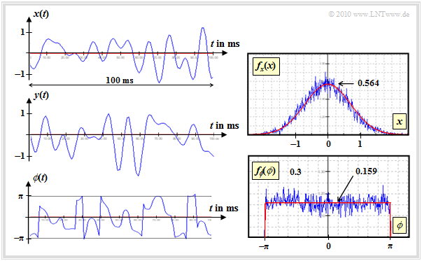
The following graphs show signal curves of $\text{100 ms}$ duration and the corresponding density functions. These are screen shots of the Windows program "Mobile Radio Channel" from the (former) practical course Simulation of digital transmission systems at the TU Munich.

$\text{Example 1:}$ In the following, exemplary signal curves for Rayleigh fading and the corresponding probability density functions are shown. These time curve representations can be interpreted as follows:

Real part, imaginary part and phase response with Rayleigh fading

The real part is Gaussian distributed (see upper right graph), as shown in the signal $x(t)$. Red is the Gaussian PDF $f_x(x)$ and blue is the histogram obtained by simulation over $10\hspace{0.05cm}000$ Samples.

The parameter used was a maximum Doppler frequency of $f_{\rm D, \ max} = 100 \ \rm Hz$. Therefore there are statistical bindings within the functions $x(t)$ and $y(t)$. More details about the Doppler effect can be found in the next chapter.

The PDF $f_y(y)$ of the imaginary part is identical to $f_x(x)$. The variance is $\sigma_x^2 =\sigma_y^2 = 0. 5 \ (=\sigma^2)$. Between $x(t)$ and $y(t)$ there are no statistical bindings; the signals are orthogonal.

The phase $\phi(t)$ is equally distributed between $\pm\pi$. As can be guessed from the jumping points in the phase function, $\phi(t)$ can also assume larger values. During the creation of the histogram, however, the ranges $(2k+1)\cdot \pi$ were projected to the value range of $-\pi$ ... $+\pi$ $(k$ integer$)$.

The equally distributed phase can be understood by means of the (not shown) 2D–PDF. This is rotationally symmetrical and accordingly there is no preferred direction:

\[f_{x,\hspace{0.02cm}y}(x, y) = \frac{1}{2\pi \cdot \sigma^2} \cdot {\rm e}^{ -(x^2 + y^2)/(2\sigma^2)} .\]

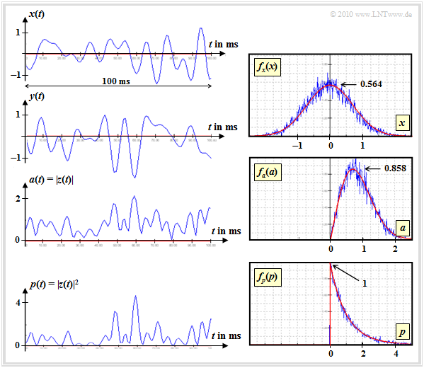
Real part, imaginary part, absolute value and square of absolute value for Rayleigh fading

$\text{Example 2}$ in continuation to $\text{Example 1}$

This graphic shows on the

left: the real part $x(t)$ and the imaginary part $y(t)$ of $z(t)$ ;
right: the PDF $f_x(x)$; the PDF $f_y(y)$ has exactly the same form.

Underneath it are the gradient and PDF

of the magnitude $a(t) =\vert z(t)\vert$ and
of the square $p(t) =a^2(t) =\vert z(t)\vert^2$.

From these descriptions it is clear:

The magnitude $a(t) =\vert z(t)\vert$ has a Rayleigh PDF ⇒ hence the name "Rayleigh fading":

\[f_a(a) = \left\{ \begin{array}{c} a/\sigma^2 \cdot {\rm e}^{-a^2/(2\sigma^2)} \\ 0 \end{array} \right.\hspace{0.15cm} \begin{array}{*{1}c} {\rm f\ddot{u}r}\hspace{0.1cm} a\hspace{-0.05cm} \ge \hspace{-0.05cm}0, \\ {\rm f\ddot{u}r}\hspace{0.1cm} a \hspace{-0.05cm}<\hspace{-0.05cm} 0. \\ \end{array} \]

For the moments of first and second order and the variance of the absolute value function $a(t)$ applies:

\[{\rm E}\big [a \big] = \sigma \cdot \sqrt {{\pi}/{2}}\hspace{0.05cm},\hspace{0.5cm}{\rm E}\big[a^2 \big] = 2 \cdot \sigma^2\]

\[ \Rightarrow \hspace{0.3cm} {\rm Var}\big[a \big] = \sigma_a^2 = \sigma^2 \cdot \left ( 2 - {\pi}/{2}\right ) \hspace{0.05cm}. \]

The PDF of the absolute value square $p(t)$ is given by nonlinear transformation the PDF $f_a(a)$ ⇒ $f_p(p)$ is exponentially distributed:

\[f_p(p) \hspace{-0.05cm}=\hspace{-0.05cm} \left\{ \begin{array}{c} (2\sigma^2)^{-1} \hspace{-0.05cm}\cdot \hspace{-0.05cm} {\rm e}^{-p^2\hspace{-0.05cm}/(2\sigma^2)} \\ 0 \end{array} \right.\hspace{0.05cm} \begin{array}{*{1}c} {\rm f\ddot{u}r}\hspace{0.05cm} p \hspace{-0.05cm}\ge \hspace{-0.05cm}0, \\ {\rm f\ddot{u}r}\hspace{0.15cm} p\hspace{-0.05cm} < \hspace{-0.05cm}0. \\ \end{array} \]

Further information about the Rayleigh–Fading can be found in the Exercise 1.3 and the Exercise 1.3Z.

Exercises to the chapter

Exercise 1.3: Rayleigh Fading

Exercise 1.3Z: Rayleigh Fading Revisited