Difference between revisions of "Theory of Stochastic Signals/Two-Dimensional Random Variables"
| Line 78: | Line 78: | ||
:$$f_{xy}(x_\mu, \hspace{0.1cm}y_\mu) = \lim_{\left.{\Delta x\rightarrow 0 \atop {\Delta y\rightarrow 0} }\right.}\frac{ {\rm Pr}\big [ (x_\mu - {\rm \Delta} x/{\rm 2} \le x \le x_\mu + {\rm \Delta} x/{\rm 2}) \cap (y_\mu - {\rm \Delta} y/{\rm 2} \le y \le y_\mu +{\rm \Delta}y/{\rm 2}) \big] }{ {\rm \Delta} \ x\cdot{\rm \Delta} y}.$$ | :$$f_{xy}(x_\mu, \hspace{0.1cm}y_\mu) = \lim_{\left.{\Delta x\rightarrow 0 \atop {\Delta y\rightarrow 0} }\right.}\frac{ {\rm Pr}\big [ (x_\mu - {\rm \Delta} x/{\rm 2} \le x \le x_\mu + {\rm \Delta} x/{\rm 2}) \cap (y_\mu - {\rm \Delta} y/{\rm 2} \le y \le y_\mu +{\rm \Delta}y/{\rm 2}) \big] }{ {\rm \Delta} \ x\cdot{\rm \Delta} y}.$$ | ||
$\rm Note$: | $\rm Note$: | ||
| − | *If the | + | *If the two-dimensional random variable is discrete, the definition must be slightly modified: |
*For the lower range limits, the "less-than-equal" sign must then be replaced by the "less-than" sign according to the section [[Theory_of_Stochastic_Signals/Cumulative_Distribution_Function#CDF_for_discrete-valued_random_variables|CDF for discrete random variables]]. }} | *For the lower range limits, the "less-than-equal" sign must then be replaced by the "less-than" sign according to the section [[Theory_of_Stochastic_Signals/Cumulative_Distribution_Function#CDF_for_discrete-valued_random_variables|CDF for discrete random variables]]. }} | ||
| − | Using this joint PDF | + | Using this joint PDF $f_{xy}(x, y)$, statistical dependencies within the two-dimensional random variable $(x,\ y)$ are also fully captured in contrast to the two one-dimensional density functions ⇒ '''marginal probability density functions''' $($or "edge probability density functions"$)$: |
:$$f_{x}(x) = \int _{-\infty}^{+\infty} f_{xy}(x,y) \,\,{\rm d}y ,$$ | :$$f_{x}(x) = \int _{-\infty}^{+\infty} f_{xy}(x,y) \,\,{\rm d}y ,$$ | ||
:$$f_{y}(y) = \int_{-\infty}^{+\infty} f_{xy}(x,y) \,\,{\rm d}x .$$ | :$$f_{y}(y) = \int_{-\infty}^{+\infty} f_{xy}(x,y) \,\,{\rm d}x .$$ | ||
| Line 116: | Line 116: | ||
*For two-dimensional random variables, the PDF volume is always equal $1$.}} | *For two-dimensional random variables, the PDF volume is always equal $1$.}} | ||
| − | ==PDF | + | ==PDF for statistically independent components== |
<br> | <br> | ||
| − | For statistically independent components $x$ | + | For statistically independent components $x$, $y$ the following holds for the joint probability according to the elementary laws of statistics if $x$ and $y$ are continuous in value: |
:$${\rm Pr} \big[(x_{\rm 1}\le x \le x_{\rm 2}) \cap( y_{\rm 1}\le y\le y_{\rm 2})\big] ={\rm Pr} (x_{\rm 1}\le x \le x_{\rm 2}) \cdot {\rm Pr}(y_{\rm 1}\le y\le y_{\rm 2}) .$$ | :$${\rm Pr} \big[(x_{\rm 1}\le x \le x_{\rm 2}) \cap( y_{\rm 1}\le y\le y_{\rm 2})\big] ={\rm Pr} (x_{\rm 1}\le x \le x_{\rm 2}) \cdot {\rm Pr}(y_{\rm 1}\le y\le y_{\rm 2}) .$$ | ||
| − | For this, independent components can also be written: | + | For this, in the case of independent components can also be written: |
:$${\rm Pr} \big[(x_{\rm 1}\le x \le x_{\rm 2}) \cap(y_{\rm 1}\le y\le y_{\rm 2})\big] =\int _{x_{\rm 1}}^{x_{\rm 2}}f_{x}(x) \,{\rm d}x\cdot \int_{y_{\rm 1}}^{y_{\rm 2}} f_{y}(y) \, {\rm d}y.$$ | :$${\rm Pr} \big[(x_{\rm 1}\le x \le x_{\rm 2}) \cap(y_{\rm 1}\le y\le y_{\rm 2})\big] =\int _{x_{\rm 1}}^{x_{\rm 2}}f_{x}(x) \,{\rm d}x\cdot \int_{y_{\rm 1}}^{y_{\rm 2}} f_{y}(y) \, {\rm d}y.$$ | ||
{{BlaueBox|TEXT= | {{BlaueBox|TEXT= | ||
| − | $\text{Definition:}$ It follows that for '''statistical independence''' the following condition must be satisfied with respect to the | + | $\text{Definition:}$ It follows that for '''statistical independence''' the following condition must be satisfied with respect to the '''two-dimensional probability density function''': |
:$$f_{xy}(x,y)=f_{x}(x) \cdot f_y(y) .$$}} | :$$f_{xy}(x,y)=f_{x}(x) \cdot f_y(y) .$$}} | ||
{{GraueBox|TEXT= | {{GraueBox|TEXT= | ||
| − | $\text{Example 2:}$ In the graph, the instantaneous values of a two-dimensional random variable are plotted as points in the $(x, y)$–plane. | + | $\text{Example 2:}$ In the graph, the instantaneous values of a two-dimensional random variable are plotted as points in the $(x,\, y)$–plane. |
| − | *Ranges with many points, which accordingly appear dark, indicate large values of the | + | *Ranges with many points, which accordingly appear dark, indicate large values of the two-dimensional PDF $f_{xy}(x,\, y)$. |
| − | *In contrast, the random variable $(x, y)$ has relatively few components in rather bright areas. | + | *In contrast, the random variable $(x,\, y)$ has relatively few components in rather bright areas. |
| − | |||
| − | |||
| − | |||
| + | [[File:P_ID153__Sto_T_4_1_S4_nochmals_neu.png |frame| Statistically independent components: $f_{xy}(x, y)$, $f_{x}(x)$ and $f_{y}(y)$]] | ||
| + | <br> | ||
The graph can be interpreted as follows: | The graph can be interpreted as follows: | ||
| − | *The marginal probability densities $f_{x}(x)$ and $f_{y}(y)$ already indicate that both $x$ and $y$ are Gaussian and zero mean, and that the random variable $x$ has a larger standard deviation than $y$ | + | *The marginal probability densities $f_{x}(x)$ and $f_{y}(y)$ already indicate that both $x$ and $y$ are Gaussian and zero mean, and that the random variable $x$ has a larger standard deviation (rms value) than $y$. |
| − | *$f_{x}(x)$ and $f_{y}(y)$ | + | *$f_{x}(x)$ and $f_{y}(y)$ do not provide information on whether or not statistical bindings exist for the random variable $(x,\, y)$. |
| − | *However, using the 2D PDF $f_{xy}(x,y)$ one can see that there are no statistical bindings between the two components $x$ and $y$ | + | *However, using the "2D-PDF" $f_{xy}(x,\, y)$ one can see that here there are no statistical bindings between the two components $x$ and $y$. |
| − | *With statistical independence, any cut through $f_{xy}(x, y)$ parallel to $y$ | + | *With statistical independence, any cut through $f_{xy}(x, y)$ parallel to $y$–axis yields a function that is equal in shape to the marginal PDF $f_{y}(y)$. Similarly, all cuts parallel to $x$–axis are equal in shape to $f_{x}(x)$. |
| − | + | *This fact is equivalent to saying that in this example $f_{xy}(x,\, y)$ can be represented as the product of the two marginal probability densities: | |
| − | *This fact is equivalent to saying that in this example $f_{xy}(x, y)$ can be represented as the product of the two marginal probability densities: $f_{xy}(x,y)=f_{x}(x) \cdot f_y(y) .$}} | + | :$$f_{xy}(x,\, y)=f_{x}(x) \cdot f_y(y) .$$}} |
| − | ==PDF | + | ==PDF for statistically dependent components== |
<br> | <br> | ||
| − | If there are statistical bindings between $x$ and $y$, then different cuts parallel to $x$– and $y$–axis, | + | If there are statistical bindings between $x$ and $y$, then different cuts parallel to $x$– and $y$–axis, resp., yield different (non-shape equivalent) functions. In this case, of course, the joint PDF cannot be described as a product of the two (one-dimensional) marginal probability densities functionseither. |
| − | [[File:P_ID156__Sto_T_4_1_S5_neu.png |right|frame|Statistically dependent components: $f_{xy}(x,y)$, $f_{x}(x)$, $f_{y}(y)$ ]] | + | {{GraueBox|TEXT= |
| − | + | $\text{Example 3:}$ The graph shows the instantaneous values of a two-dimensional random variable in the $(x, y)$–plane. | |
| − | + | [[File:P_ID156__Sto_T_4_1_S5_neu.png |right|frame|Statistically dependent components: $f_{xy}(x, y)$, $f_{x}(x)$, $f_{y}(y)$ ]] | |
| − | *The | + | <br>Now, unlike $\text{Example 2}$ there are statistical bindings between $x$ and $y$. |
| + | *The two-dimensional random variable takes all "2D" values with equal probability in the parallelogram drawn in blue. | ||
*No values are possible outside the parallelogram. | *No values are possible outside the parallelogram. | ||
| − | One recognizes from this representation: | + | <br>One recognizes from this representation: |
| − | + | #Integration over $f_{xy}(x, y)$ parallel to the $x$–axis leads to the triangular marginal PDF $f_{y}(y)$, integration parallel to $y$–axis to the trapezoidal PDF $f_{x}(x)$. | |
| − | + | #From the joint PDF $f_{xy}(x, y)$ it can already be guessed that for each $x$–value on statistical average a different $y$–value is to be expected. | |
| − | + | #This means that the components $x$ and $y$ are statistically dependent on each other. }} | |
==Expected values of two-dimensional random variables== | ==Expected values of two-dimensional random variables== | ||
Revision as of 11:48, 23 January 2022
Contents
- 1 # OVERVIEW OF THE FOURTH MAIN CHAPTER #
- 2 Properties and examples
- 3 Joint probability density function
- 4 Two-dimensional cumulative distribution function
- 5 PDF for statistically independent components
- 6 PDF for statistically dependent components
- 7 Expected values of two-dimensional random variables
- 8 Correlation coefficient
- 9 Correlation line
- 10 Exercises for the chapter
# OVERVIEW OF THE FOURTH MAIN CHAPTER #
$\Rightarrow \hspace{0.5cm}\text{We are just beginning the English translation of this chapter.}$
Now random variables with statistical bindings are treated and illustrated by typical examples.
After the general description of two-dimensional random variables, we turn to
- the "auto-correlation function",
- the cross-correlation function"
- and the associated spectral functions $($"power-spectral density", "cross power-spectral density"$)$.
Specifically, this chapter covers:
- the statistical description of »two-dimensional random variables« using the »joint PDF«,
- the difference between »statistical dependence« and »correlation«,
- the classification features »stationarity« and »ergodicity« of stochastic processes,
- the definitions of »auto-correlation function« $\rm (ACF)$ and »power-spectral density« $\rm (PSD)$,
- the definitions of »cross-correlation function« $\rm (CCF)$ and »cross power-spectral density« $\rm (C–PSD)$,
- the numerical determination of all these variables in the two- and multi-dimensional case.
Properties and examples
As a transition to the "correlation functions" we now consider two random variables $x$ and $y$, between which statistical dependences exist.
Each of these two random variables can be described on its own with the introduced characteristic variables corresponding
- to the second main chapter ⇒ Discrete Random Variables
- and the third main chapter ⇒ Continuous Random Variables.
$\text{Definition:}$ To describe the statistical dependences between two variables $x$ and $y$, it is convenient to combine the two components
into one "two-dimensional random variable" or "2D random variable" $(x, y)$.
- The individual components can be signals such as the real and imaginary parts of a phase modulated signal.
- But there are a variety of two-dimensional random variables in other domains as well, as the following example will show.
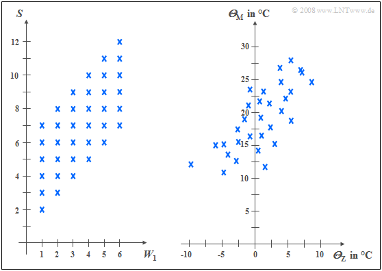
$\text{Example 1:}$ The left diagram is from the random experiment "Throwing two dice".
- Plotted to the right is the number of the first die $(W_1)$,
- plotted to the top is the sum $S$ of both dice.
The two components here are each discrete random variables between which there are statistical dependencies:
- If $W_1 = 1$, then the sum $S$ can only take values between $2$ and $7$, each with equal probability.
- In contrast, for $W_1 = 6$ all values between $7$ and $12$ are possible, also with equal probability.
In the right diagram, the maximum temperatures of the $31$ days in May 2002 of Munich (to the top) and the mountain "Zugspitze" (to the right) are contrasted. Both random variables are continuous in value:
- Although the measurement points are about $\text{100 km}$ apart, and on the Zugspitze, due to the different altitudes $($nearly $3000$ versus $520$ meters$)$ is on average about $20$ degrees colder than in Munich, one recognizes nevertheless a certain statistical dependence between the two random variables ${\it Θ}_{\rm M}$ and ${\it Θ}_{\rm Z}$.
- If it is warm in Munich, then pleasant temperatures are also more likely to be expected on the Zugspitze. However, the relationship is not deterministic: The coldest day in May 2002 was a different day in Munich than the coldest day on the Zugspitze.
Joint probability density function
We restrict ourselves here mostly to continuous valued random variables.
- However, sometimes the peculiarities of two-dimensional discrete random variables are discussed in more detail.
- Most of the characteristics previously defined for one-dimensional random variables can be easily extended to two-dimensional variables.
$\text{Definition:}$
The probability density function $\rm (PDF)$ of the two-dimensional random variable at the location $(x_\mu,\hspace{0.1cm} y_\mu)$ ⇒ "joint PDF" or "2D–PDF"
is an extension of the one-dimensional PDF $(∩$ denotes logical "AND" operation$)$:
- $$f_{xy}(x_\mu, \hspace{0.1cm}y_\mu) = \lim_{\left.{\Delta x\rightarrow 0 \atop {\Delta y\rightarrow 0} }\right.}\frac{ {\rm Pr}\big [ (x_\mu - {\rm \Delta} x/{\rm 2} \le x \le x_\mu + {\rm \Delta} x/{\rm 2}) \cap (y_\mu - {\rm \Delta} y/{\rm 2} \le y \le y_\mu +{\rm \Delta}y/{\rm 2}) \big] }{ {\rm \Delta} \ x\cdot{\rm \Delta} y}.$$
$\rm Note$:
- If the two-dimensional random variable is discrete, the definition must be slightly modified:
- For the lower range limits, the "less-than-equal" sign must then be replaced by the "less-than" sign according to the section CDF for discrete random variables.
Using this joint PDF $f_{xy}(x, y)$, statistical dependencies within the two-dimensional random variable $(x,\ y)$ are also fully captured in contrast to the two one-dimensional density functions ⇒ marginal probability density functions $($or "edge probability density functions"$)$:
- $$f_{x}(x) = \int _{-\infty}^{+\infty} f_{xy}(x,y) \,\,{\rm d}y ,$$
- $$f_{y}(y) = \int_{-\infty}^{+\infty} f_{xy}(x,y) \,\,{\rm d}x .$$
These two marginal probability density functions $f_x(x)$ and $f_y(y)$
- provide only statistical information about the individual components $x$ and $y$, resp.
- but not about the statistical bindings between them.
Two-dimensional cumulative distribution function
$\text{Definition:}$ Like the "2D–PDF", the 2D cumulative distribution function is merely a useful extension of the one-dimensional distribution function $\rm (CDF)$:
- $$F_{xy}(r_{x},r_{y}) = {\rm Pr}\big [(x \le r_{x}) \cap (y \le r_{y}) \big ] .$$
The following similarities and differences between the "1D–CDF" and the 2D–CDF" emerge:
- The functional relationship between two-dimensional PDF and two-dimensional CDF is given by integration as in the one-dimensional case, but now in two dimensions. For continuous valued random variables:
- $$F_{xy}(r_{x},r_{y})=\int_{-\infty}^{r_{y}} \int_{-\infty}^{r_{x}} f_{xy}(x,y) \,\,{\rm d}x \,\, {\rm d}y .$$
- Inversely, the probability density function can be given from the cumulative distribution function by partial differentiation to $r_{x}$ and $r_{y}$:
- $$f_{xy}(x,y)=\frac{{\rm d}^{\rm 2} F_{xy}(r_{x},r_{y})}{{\rm d} r_{x} \,\, {\rm d} r_{y}}\Bigg|_{\left.{r_{x}=x \atop {r_{y}=y}}\right.}.$$
- Relative to the two-dimensional cumulative distribution function $F_{xy}(r_{x}, r_{y})$ the following limits apply:
- $$F_{xy}(-\infty,-\infty) = 0,$$
- $$F_{xy}(r_{\rm x},+\infty)=F_{x}(r_{x} ),$$
- $$F_{xy}(+\infty,r_{y})=F_{y}(r_{y} ) ,$$
- $$F_{xy} (+\infty,+\infty) = 1.$$
- From the last equation $($infinitely large $r_{x}$ and $r_{y})$ we obtain the normalization condition for the "2D– PDF":
- $$\int_{-\infty}^{+\infty} \int_{-\infty}^{+\infty} f_{xy}(x,y) \,\,{\rm d}x \,\,{\rm d}y=1 . $$
$\text{Conclusion:}$ Note the significant difference between one-dimensional and two-dimensional random variables:
- For one-dimensional random variables, the area under the PDF always yields the value $1$.
- For two-dimensional random variables, the PDF volume is always equal $1$.
PDF for statistically independent components
For statistically independent components $x$, $y$ the following holds for the joint probability according to the elementary laws of statistics if $x$ and $y$ are continuous in value:
- $${\rm Pr} \big[(x_{\rm 1}\le x \le x_{\rm 2}) \cap( y_{\rm 1}\le y\le y_{\rm 2})\big] ={\rm Pr} (x_{\rm 1}\le x \le x_{\rm 2}) \cdot {\rm Pr}(y_{\rm 1}\le y\le y_{\rm 2}) .$$
For this, in the case of independent components can also be written:
- $${\rm Pr} \big[(x_{\rm 1}\le x \le x_{\rm 2}) \cap(y_{\rm 1}\le y\le y_{\rm 2})\big] =\int _{x_{\rm 1}}^{x_{\rm 2}}f_{x}(x) \,{\rm d}x\cdot \int_{y_{\rm 1}}^{y_{\rm 2}} f_{y}(y) \, {\rm d}y.$$
$\text{Definition:}$ It follows that for statistical independence the following condition must be satisfied with respect to the two-dimensional probability density function:
- $$f_{xy}(x,y)=f_{x}(x) \cdot f_y(y) .$$
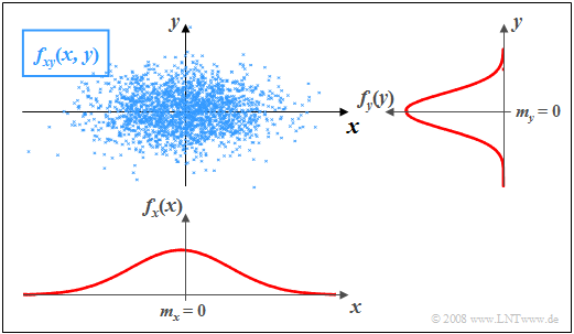
$\text{Example 2:}$ In the graph, the instantaneous values of a two-dimensional random variable are plotted as points in the $(x,\, y)$–plane.
- Ranges with many points, which accordingly appear dark, indicate large values of the two-dimensional PDF $f_{xy}(x,\, y)$.
- In contrast, the random variable $(x,\, y)$ has relatively few components in rather bright areas.
The graph can be interpreted as follows:
- The marginal probability densities $f_{x}(x)$ and $f_{y}(y)$ already indicate that both $x$ and $y$ are Gaussian and zero mean, and that the random variable $x$ has a larger standard deviation (rms value) than $y$.
- $f_{x}(x)$ and $f_{y}(y)$ do not provide information on whether or not statistical bindings exist for the random variable $(x,\, y)$.
- However, using the "2D-PDF" $f_{xy}(x,\, y)$ one can see that here there are no statistical bindings between the two components $x$ and $y$.
- With statistical independence, any cut through $f_{xy}(x, y)$ parallel to $y$–axis yields a function that is equal in shape to the marginal PDF $f_{y}(y)$. Similarly, all cuts parallel to $x$–axis are equal in shape to $f_{x}(x)$.
- This fact is equivalent to saying that in this example $f_{xy}(x,\, y)$ can be represented as the product of the two marginal probability densities:
- $$f_{xy}(x,\, y)=f_{x}(x) \cdot f_y(y) .$$
PDF for statistically dependent components
If there are statistical bindings between $x$ and $y$, then different cuts parallel to $x$– and $y$–axis, resp., yield different (non-shape equivalent) functions. In this case, of course, the joint PDF cannot be described as a product of the two (one-dimensional) marginal probability densities functionseither.
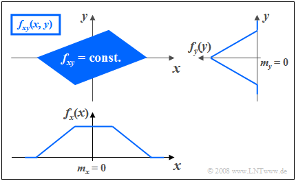
$\text{Example 3:}$ The graph shows the instantaneous values of a two-dimensional random variable in the $(x, y)$–plane.
Now, unlike $\text{Example 2}$ there are statistical bindings between $x$ and $y$.
- The two-dimensional random variable takes all "2D" values with equal probability in the parallelogram drawn in blue.
- No values are possible outside the parallelogram.
One recognizes from this representation:
- Integration over $f_{xy}(x, y)$ parallel to the $x$–axis leads to the triangular marginal PDF $f_{y}(y)$, integration parallel to $y$–axis to the trapezoidal PDF $f_{x}(x)$.
- From the joint PDF $f_{xy}(x, y)$ it can already be guessed that for each $x$–value on statistical average a different $y$–value is to be expected.
- This means that the components $x$ and $y$ are statistically dependent on each other.
Expected values of two-dimensional random variables
A special case of statistical dependence is correlation.
$\text{Definition:}$ Under correlation one understands a linear dependence between the individual components $x$ and $y$.
- Correlated random variables are thus always also statistically dependent.
- But not every statistical dependence implies correlation at the same time
.
To quantitatively capture correlation, one uses various expected values of the 2D random variable $(x, y)$.
These are defined analogously to the one-dimensional case.
- according to Chapter 2 (for discrete value random variables).
- bzw. Chapter 3 (for continuous value random variables):
$\text{Definition:}$ For the (non-centered) moments the relation holds:
- $$m_{kl}={\rm E}\big[x^k\cdot y^l\big]=\int_{-\infty}^{+\infty}\hspace{0.2cm}\int_{-\infty}^{+\infty} x\hspace{0.05cm}^{k} \cdot y\hspace{0.05cm}^{l} \cdot f_{xy}(x,y) \, {\rm d}x\, {\rm d}y.$$
Thus, the two linear means are $m_x = m_{10}$ and $m_y = m_{01}.$
$\text{definition:}$ The $m_x$ and $m_y$ related central moments respectively are:
- $$\mu_{kl} = {\rm E}\big[(x-m_{x})\hspace{0.05cm}^k \cdot (y-m_{y})\hspace{0.05cm}^l\big] .$$
In this general definition equation, the variances $σ_x^2$ and $σ_y^2$ of the two individual components are included by $\mu_{20}$ and $\mu_{02}$ respectively.
$\text{Definition:}$ Of particular importance is the covariance $(k = l = 1)$, which is a measure of the linear statistical dependence between the random variables $x$ and $y$ :
- $$\mu_{11} = {\rm E}\big[(x-m_{x})\cdot(y-m_{y})\big] = \int_{-\infty}^{+\infty} \int_{-\infty}^{+\infty} (x-m_{x}) \cdot (y-m_{y})\cdot f_{xy}(x,y) \,{\rm d}x \, {\rm d}y .$$
In the following, we also denote the covariance $\mu_{11}$ in part by $\mu_{xy}$, if the covariance refers to the random variables $x$ and $y$
Notes:
- The covariance $\mu_{11}=\mu_{xy}$ is related to the non-centered moment $m_{11} = m_{xy} = {\rm E}\big[x \cdot y\big]$ as follows:
- $$\mu_{xy} = m_{xy} -m_{x }\cdot m_{y}.$$
- This equation is enormously advantageous for numerical evaluations, since $m_{xy}$, $m_x$ and $m_y$ can be found from the sequences $〈x_v〉$ and $〈y_v〉$ in a single run.
- On the other hand, if one were to calculate the covariance $\mu_{xy}$ according to the above definition equation, one would have to find the mean values $m_x$ and $m_y$ in a first run and could then only calculate the expected value ${\rm E}\big[(x - m_x) \cdot (y - m_y)\big]$ in a second run.
$\text{Example 4:}$ In the first two rows of the table, the respective first elements of two random sequences $〈x_ν〉$ and $〈y_ν〉$ are entered. In the last row, the respective products $x_ν - y_ν$ are given.
- By averaging over the ten sequence elements in each case, one obtains
- $$m_x =0.5,\ \ m_y = 1, \ \ m_{xy} = 0.69.$$
- This directly results in the value for the covariance:
- $$\mu_{xy} = 0.69 - 0.5 · 1 = 0.19.$$
Without knowledge of the equation $\mu_{xy} = m_{xy} - m_x\cdot m_y$ one would have had to first determine the mean values $m_x$ and $m_y$ in the first run,
in order to then determine the covariance $\mu_{xy}$ as the expected value of the product of the zero mean variables in a second run.
Correlation coefficient
With statistical independence of the two components $x$ and $y$ the covariance $\mu_{xy} \equiv 0$. This case has already been considered in $\text{Example 2}$ on the PDF and CDF for statistically independent components page.
- But the result $\mu_{xy} = 0$ is also possible for statistically dependent components $x$ and $y$ namely when they are uncorrelated, i.e. linearly independent .
- The statistical dependence is then not of first order, but of higher order, for example corresponding to the equation $y=x^2.$
One speaks of complete correlation when the (deterministic) dependence between $x$ and $y$ is expressed by the equation $y = K · x$ . Then the covariance is given by:
- $\mu_{xy} = σ_x · σ_y$ with positive value of $K$,
- $\mu_{xy} = - σ_x · σ_y$ with negative $K$–value.
Therefore, instead of covariance, one often uses the so-called correlation coefficient as a descriptive variable.
$\text{Definition:}$ The correlation coefficient is the quotient of the covariance $\mu_{xy}$ and the product of the rms values $σ_x$ and $σ_y$ of the two components:
- $$\rho_{xy}=\frac{\mu_{xy} }{\sigma_x \cdot \sigma_y}.$$
The correlation coefficient $\rho_{xy}$ has the following properties:
- Because of normalization, $-1 \le ρ_{xy} ≤ +1$ always holds.
- If the two random variables $x$ and $y$ are uncorrelated, then $ρ_{xy} = 0$.
- For strict linear dependence between $x$ and $y$ is $ρ_{xy}= ±1$ ⇒ complete correlation.
- A positive correlation coefficient means that when $x$ is larger, on statistical average $y$ is also larger than when $x$ is smaller.
- In contrast, a negative correlation coefficient expresses that $y$ becomes smaller on average as $x$ increases.
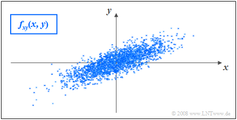
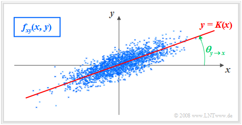
$\text{Example 5:}$ The following conditions apply:
- The considered components $x$ and $y$ each have a Gaussian PDF.
- The two standard deviations are different $(σ_y < σ_x)$.
- The correlation coefficient is $ρ_{xy} = 0.8$.
Unlike the Example 2 with statistically independent components ⇒ $ρ_{xy} = 0$ $($drotz $σ_y < σ_x)$ one recognizes that here with larger $x$-value on statistical average also $y$ is larger than with smaller $x$.
Correlation line
$\text{Definition:}$ A correlation line is the straight line $y = K(x)$ in the $(x, y)$–plane through the "midpoint" $(m_x, m_y)$. Sometimes this straight line is also called regression line .
The correlation line has the following properties:
- The mean square deviation(error???) from this straight line - viewed in $y$–direction and averaged over all $N$ points - is minimal:
- $$\overline{\varepsilon_y^{\rm 2} }=\frac{\rm 1}{N} \cdot \sum_{\nu=\rm 1}^{N}\; \;\big [y_\nu - K(x_{\nu})\big ]^{\rm 2}={\rm minimum}.$$
- The correlation straight line can be interpreted as a kind of "statistical symmetry axis" . The equation of the straight line is:
- $$y=K(x)=\frac{\sigma_y}{\sigma_x}\cdot\rho_{xy}\cdot(x - m_x)+m_y.$$
The angle taken by the correlation line to the $x$–axis is:
- $$\theta_{y\hspace{0.05cm}\rightarrow \hspace{0.05cm}x}={\rm arctan}\ (\frac{\sigma_{y} }{\sigma_{x} }\cdot \rho_{xy}).$$
By this nomenclature it should be made clear that we are dealing here with the regression of $y$ on $x$ .
- The regression in the opposite direction - that is, from $x$ to $y$ - on the other hand, means the minimization of the mean square deviation in $x$ direction.
- The interactive applet Correlation Coefficient and Regression Line illustrates that in general $($if $σ_y \ne σ_x)$ for the regression of $x$ on $y$ will result in a different angle and thus a different regression line:
- $$\theta_{x\hspace{0.05cm}\rightarrow \hspace{0.05cm} y}={\rm arctan}\ (\frac{\sigma_{x}}{\sigma_{y}}\cdot \rho_{xy}).$$
Exercises for the chapter
Exercise 4.1: Triangular (x, y) Area
Exercise 4.1Z: Appointment to Breakfast
Exercise 4.2: Triangle Area again
Exercise 4.2Z: Correlation between "x" and "e to the Power of x"
Exercise 4.3: Algebraic and Modulo Sum
Exercise 4.3Z: Dirac-shaped 2D PDF
