Nonlinear Distortions

Properties of nonlinear systems

The system description by means of the frequency response $H(f)$ and/or impulse response $h(t)$ is only possible for an LTI System . However, if the system also contains nonlinear components, as it is assumed for this chapter, no frequency response and no impulse response can be stated, and the model must be designed in a more general way.

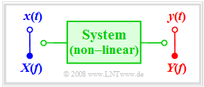
Description of a nonlinear systems

Also, in this nonlinear system we denote the signals at the input and output by $x(t)$ and $y(t)$ respectively, and the corresponding spectral functions by $X(f)$ and $Y(f)$.

An observer will note the following here:

The transmission characteristics are now also dependent on the amplitude of the input signal . If $x(t)$ results in the output signal $y(t)$, it can now no longer be concluded that the input signal $K · x(t)$ will always result in the signal $K · y(t)$ .
This also implies that the superposition principle is no longer applicable . Consequently, the result $x_1(t) + x_2(t) ⇒ y_1(t) + y_2(t)$ cannot be reasoned from the two correspondences $x_1(t) ⇒ y_1(t)$ and $x_2(t) ⇒ y_2(t)$ .
Due to nonlinearities new frequencies occur. If $x(t)$ is a harmonic oscillation with the frequency $f_0$, the output signal $y(t)$ also contains components at multiples of $f_0$. In communications engineering, these are referred to as harmonics.
In practice, an information signal usually contains many frequency components. The harmonics of the low-frequency signal components now fall into the range of higher-frequency useful components. This results in nonreversible signal falsifications.

Before mentioning "constellations which result in nonlinear distortions" at the end of the section the problem of nonlinear distortions is captured mathematically.

We assume here that the system has no memory so that the output value $y = y(t_0)$ depends only on the instantaneous input value $x = x(t_0)$
but not on the signal curve $x(t)$ for $t < t_0$.

Description of nonlinear systems

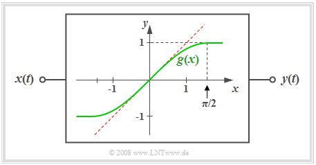
$\text{Definition:}$ A system is said to be nonlinear if the following relationship exists between the signal value $x = x(t)$ at the input and the output $y = y(t)$ : $$y = g(x) \ne {\rm const.} \cdot x.$$ The curve shape $y = g(x)$ is called the nonlinear characteristic curve of the system.

Nonlinear characteristic curve

In the diagram, as an example, the green curve is the nonlinear characteristic curve $y = g(x)$ which is shaped according to the first quarter of a sine function.
The special case of a linear system with the characteristic curve $y = x$ can be seen dashed in red.

Since every characteristic curve can be developed into a Taylor series around the operating point the output signal can also be represented as follows: $$y(t) = \sum_{i=0}^{\infty}\hspace{0.1cm} c_i \cdot x^{i}(t) = c_0 + c_1 \cdot x(t) + c_2 \cdot x^{2}(t) + c_3 \cdot x^{3}(t) + \hspace{0.05cm}\text{...}$$ If $x(t)$ has a unit – for exmple "Volt” –, then the coefficients of the Taylor series also have appropriate and different units:

$c_0$ with $\rm V$,
$c_1$ without units,
$c_2$ with $\rm 1/V$, etc.

In the above diagram, the operating point is identical to the zero point and $c_0 = 0$ holds.

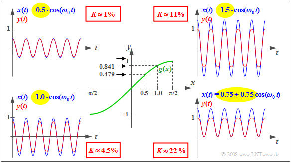
$\text{Example 1:}$ The properties of nonlinear systems listed on the first page of this section are illustrated here using the characteristic curve $y = g(x) = \sin(x)$ shown in the centre of the diagram.

Here, the direct (DC) signal $x(t) = 0.5$ results in the constant output signal $y(t) = 0.479$ .
For $x(t) = 1$ the input signal results in the output signal $y(t) = 0.841 ≠ 2 · 0.479$.

Thus, doubling $x(t)$ does not cause the doubling of $y(t)$ ⇒ the superposition principle is violated.

Effects of a nonlinear characteristic curve

The outer diagrams show – each in blue – cosine-shaped input signals $x(t)$ with different amplitudes $A$ and the corresponding distorted output signals $y(t)$ in red. It can be seen that the nonlinear distortions increase with increasing amplitude, which are quantified by the distortion factor $K$ defined on the next page.

The diagram on the upper right-hand corner for $A = 1.5$ clearly shows that $y(t)$ is no longer cosine-shaped; the half-waves run rounder than the ones of the cosine function.
But also for $A = 0.5$ and $A = 1.0$ the signals $y(t)$ deviate - although less strongly - from the cosine form due to the harmonics. That is, new frequency components at multiples of the cosine frequency $f_0$ arise.

In the picture on the bottom right-hand corner the characteristic curve is operated unilaterally due to an additional direct component. Now an unbalance in the signal $y(t)$ can be seen, too. The lower half-wave is more peaked than the upper one. The distortion factor here is $K \approx 22\%$.

The distortion factor

Definition of the distortion factor

To quantitatively capture the nonlinear distortions we assume that the input signal $x(t)$ is cosine-shaped with the amplitude $A_x$ .

The output signal contains harmonics due to the nonlinear distortions and the following is generally true: $$y(t) = A_0 + A_1 \cdot \cos(\omega_0 t) + A_2 \cdot \cos(2\omega_0 t) + A_3 \cdot \cos(3\omega_0 t) + \hspace{0.05cm}...$$

$\text{Definition:}$ With these amplitude values $A_i$ the equation for the distortion factor is:

$$K = \frac {\sqrt{A_2^2+ A_3^2+ A_4^2+ \hspace{0.05cm}\text{...} } }{A_1} = \sqrt{K_2^2+ K_3^2+K_4^2+ \hspace{0.05cm}\text{...} }.$$

In the second equation

$K_2 = A_2/A_1$ denotes the distortion factor of second order,
$K_3 = A_3/A_1$ denotes the distortion factor of third order, etc.

It is explicitly pointed out that the amplitude $A_x$ of the input signal is not taken into account when computing the distortion factor. Also a resulting direct (DC) component $A_0$ is not taken into account.

In the last section of $\text{Example 1}$ the distortion factors were specified with values between about $1\%$ and $20\%$ .

These values are already significantly above the distortion factors of low-cost audio equipment, for which $K < 0.1\%$ applies.
In HiFi equipment, particular emphasis is placed on linearity and a very low distortion factor is also reflected in the price.

A comparison with the page Consideration of Attenuation and Runtime reveals that for the special case of a cosine-shaped input signal the signal–to–distortion–power ratio defined is equal to the reciprocal of the distortion factor squared:

$$\rho_{\rm V} = \frac{ \alpha^2 \cdot P_{x}}{P_{\rm V}} = \left(\frac{ A_{1}}{A_x} \right)^2 \cdot \frac{ {1}/{2} \cdot A_{x}^2}{{1}/{2} \cdot (A_{2}^2 + A_{3}^2 + A_{4}^2 + \hspace{0.05cm}...) } = \frac{1}{K^2}\hspace{0.05cm}.$$

Influence of a nonlinearity on a cosine signal

$\text{Example 2:}$ We now consider an averaged cosine signal:

$$x(t) = {1}/{2} + {1}/{2}\cdot \cos (\omega_0 \cdot t).$$

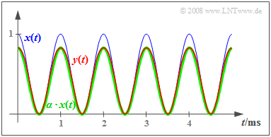
$x(t)$ takes values between $0$ and $1$ , and is drawn as the blue curve. The signal power is

$$P_x = 1/4 + 1/8 = 0.375.$$

If we apply this signal to a nonlinearity with the characteristic curve

$$y=g(x) = \sin(x) \approx x - {x^3}/{6} \hspace{0.05cm},$$

then the output signal is:

$$y(t) = A_0 + A_1 \cdot \cos (\omega_0 \cdot t)+ A_2 \cdot \cos (2\omega_0 \cdot t)+ A_3 \cdot \cos (3\omega_0 \cdot t)\hspace{0.05cm},$$

$$\Rightarrow \hspace{0.3cm} A_0 = {86}/{192},\hspace{0.3cm}A_1 = {81}/{192},\hspace{0.3cm}A_2 = - {6}/{192},\hspace{0.3cm}A_3 = - {1}/{192}\hspace{0.05cm}.$$

The trigonometric transformations for $\cos^2(α)$ and $\cos^3(α)$ were used to calculate the Fourier coefficients. The distortion factor is thus given by

$$K = \frac {\sqrt{A_2^{\hspace{0.05cm}2} + A_3^{\hspace{0.05cm}2} } }{A_1}\approx 7.5\%\hspace{0.05cm}.$$

It can be further seen that the signal $y(t)$ sketched in red is almost equal to the signal $α · x(t)$ sketched in green with $α = \sin(1) ≈ 5/6$ .

Defining the error signal as $ε_1(t) = y(t) - α · x(t)$, with its power

$$P_{\varepsilon 1} = \frac {(80-86)^2}{192^2} + \frac {6^2 + (-1)^2}{2 \cdot 192^2}\approx 1.48 \cdot 10^{-3}$$

the following is obtained for the signal–to–noise–power ratio:

$$\rho_{{\rm V} 1} = \frac {\alpha^2 \cdot P_x}{P_{\varepsilon 1} } = \frac {(5/6)^2 \cdot 0.375}{1.48 \cdot 10^{-3} }\approx 176 = {1}/{K^2}\hspace{0.05cm}.$$

In contrast, the SNR is significantly lower if we do not consider the attenuation factor, that is, if we assume the error signal $ε_2 = y(t) - x(t)$ :

$$P_{\varepsilon 2} = \frac {(86-96)^2}{192^2} + \frac {(81-96)^2 + 6^2 + (-1)^2}{2 \cdot 192^2}\approx 6.3 \cdot 10^{-3} \hspace{0.3cm} \Rightarrow \hspace{0.3cm}\rho_{{\rm V} 2} = \frac { P_x}{P_{\varepsilon 2}}= \frac {0.375}{6.3 \cdot 10^{-3}} \approx 60 \hspace{0.05cm}.$$

Clirr measurement

A major disadvantage of the definition of the distortion factor is the thereby specification to cosine-shaped test signals, i.e. to conditions remote from reality.

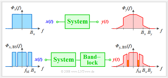
In the so-called clirr measurement the signal to be transmitted $x(t)$ is modelled by white noise with the noise power density ${\it \Phi}_x(f)$.
In addition, a narrow band-stop filter $\rm (BS)$ with centre frequency $f_{\rm M}$ and (very small) bandwidth $B_{\rm BS}$ is introduced into the system.

Principle of clirr measurement

In a linear system, the output spectrum ${\it \Phi}_y(f)$ would not be wider than $B_x$ and also in the region around $f_{\rm M}$ there would be no components.

These result solely from frequency conversion products (intermodulation components) of different spectral components, i.e. from nonlinear distortions.

By varying the centre frequency $f_{\rm M}$ and integrating over all these small interfering components the distortion power can thus be determined. More details on this method can be found, for example, in [Kam04]^[1].

Constellations which result in nonlinear distortions

As an example of the occurrence of nonlinear distortions in analog message transmission systems some constellations which result in such distortions shall be mentioned here. In terms of content, this anticipates the book Modulation Methods.

General block diagram of a message transmission system

Nonlinear distortions of the sink signal $v(t)$ with respect to the source signal $q(t)$ occur when

nonlinear distortions already occur on the channel – i.e. with respect to the transmit signal $s(t)$ and the receive signal $r(t)$,
an envelope demodulator is used for Double-Sideband Amplitude Modulation (ZSB–AM) with modulation factor $m > 1$,
for ZSB–AM and envelope demodulation there is a linearly distorting channel, even with a modulation factor $m < 1$,
the combination of single-sideband–AM and Envelope Demodulation is used (regardless of the sideband–to–carrier ratio),
an Angle Modulation (generic term for frequency and phase modulation) is applied and the available bandwidth is finite.