Difference between revisions of "Modulation Methods/Spreading Sequences for CDMA"
m (Text replacement - "power density spectrum" to "power-spectral density") |
|||
| (14 intermediate revisions by 3 users not shown) | |||
| Line 2: | Line 2: | ||
{{Header | {{Header | ||
|Untermenü=Multiple Access Methods | |Untermenü=Multiple Access Methods | ||
| − | |Vorherige Seite= | + | |Vorherige Seite=Direct-Sequence Spread Spectrum Modulation |
| − | |Nächste Seite= | + | |Nächste Seite=Error Probability of Direct-Sequence Spread Spectrum Modulation |
}} | }} | ||
==Properties of the correlation functions== | ==Properties of the correlation functions== | ||
| Line 10: | Line 10: | ||
{{BlaueBox|TEXT= | {{BlaueBox|TEXT= | ||
| − | $\text{Definition:}$ Considering two ergodic processes with model functions $x(t)$ and $y(t)$, the following applies to their [[Theory_of_Stochastic_Signals/ | + | $\text{Definition:}$ Considering two ergodic processes with model functions $x(t)$ and $y(t)$, the following applies to their [[Theory_of_Stochastic_Signals/Cross-Correlation_Function_and_Cross_Power-Spectral_Density#Definition_of_the_cross-correlation_function|$\text{cross-correlation function}$]] $\rm (CCF)$: |
:$$\varphi_{xy}(\tau)=\overline{x(t)\cdot y(t+\tau)}=\lim_{T_{\rm M}\to\infty}\,\frac{1}{T_{\rm M} }\cdot\int^{T_{\rm M}/{\rm 2} }_{-T_{\rm M}/{\rm 2} }x(t)\cdot y(t+\tau)\,\,\rm d \it t.$$ | :$$\varphi_{xy}(\tau)=\overline{x(t)\cdot y(t+\tau)}=\lim_{T_{\rm M}\to\infty}\,\frac{1}{T_{\rm M} }\cdot\int^{T_{\rm M}/{\rm 2} }_{-T_{\rm M}/{\rm 2} }x(t)\cdot y(t+\tau)\,\,\rm d \it t.$$ | ||
The line crossing over indicates a "time averaging."}} | The line crossing over indicates a "time averaging."}} | ||
| Line 23: | Line 23: | ||
{{BlaueBox|TEXT= | {{BlaueBox|TEXT= | ||
$\text{Definition:}$ | $\text{Definition:}$ | ||
| − | If we set $y(t) = x(t)$ in the above equation, we arrive at the [[Theory_of_Stochastic_Signals/Auto-Correlation_Function_(ACF)| | + | If we set $y(t) = x(t)$ in the above equation, we arrive at the [[Theory_of_Stochastic_Signals/Auto-Correlation_Function_(ACF)|$\text{auto-correlation function}$]] $\rm (ACF)$ |
:$$ \varphi_{xx}(\tau)=\overline{x(t)\cdot x(t+\tau)}=\lim_{T_{\rm M}\to\infty}\,\frac{1}{T_{\rm M} }\cdot\int^{T_{\rm M}/{\rm 2} }_{-T_{\rm M}/{\rm 2} }x(t)\cdot x(t+\tau)\,\,\rm d \it t$$ | :$$ \varphi_{xx}(\tau)=\overline{x(t)\cdot x(t+\tau)}=\lim_{T_{\rm M}\to\infty}\,\frac{1}{T_{\rm M} }\cdot\int^{T_{\rm M}/{\rm 2} }_{-T_{\rm M}/{\rm 2} }x(t)\cdot x(t+\tau)\,\,\rm d \it t$$ | ||
with the following properties: | with the following properties: | ||
| Line 35: | Line 35: | ||
The auto-correlation function and cross-correlation function describe the internal bindings and the mutual statistical dependencies in the time domain. The corresponding description functions in the frequency domain are | The auto-correlation function and cross-correlation function describe the internal bindings and the mutual statistical dependencies in the time domain. The corresponding description functions in the frequency domain are | ||
| − | *the [[Theory_of_Stochastic_Signals/ | + | *the [[Theory_of_Stochastic_Signals/Power-Spectral_Density|$\text{power-spectral density}$]] ${\it Φ}_{xx}(f)$, as well as |
| − | *the [[Theory_of_Stochastic_Signals/ | + | *the [[Theory_of_Stochastic_Signals/Cross-Correlation_Function_and_Cross_Power-Spectral_Density#Cross_power-spectral_density|$\text{cross power-spectral density}$]] ${\it Φ}_{xy}(f)$. |
| − | For ergodic processes, these are obtained as the [[Signal_Representation/ | + | For ergodic processes, these are obtained as the [[Signal_Representation/Fourier_Transform_and_its_Inverse#Fourier_transform|$\text{Fourier transforms}$]] of ACF and CCF: |
:$${\it \Phi}_{xx}(f) \hspace{0.2cm} \bullet\!\!-\!\!\!-\!\!\!-\!\!\circ\, \hspace{0.2cm}\varphi_{xx}(\tau)\hspace{0.05cm} ,\hspace{0.3cm} {\it \Phi}_{xy}(f) \hspace{0.2cm} \bullet\!\!-\!\!\!-\!\!\!-\!\!\circ\, \hspace{0.2cm}\varphi_{xy}(\tau)\hspace{0.05cm}.$$ | :$${\it \Phi}_{xx}(f) \hspace{0.2cm} \bullet\!\!-\!\!\!-\!\!\!-\!\!\circ\, \hspace{0.2cm}\varphi_{xx}(\tau)\hspace{0.05cm} ,\hspace{0.3cm} {\it \Phi}_{xy}(f) \hspace{0.2cm} \bullet\!\!-\!\!\!-\!\!\!-\!\!\circ\, \hspace{0.2cm}\varphi_{xy}(\tau)\hspace{0.05cm}.$$ | ||
| − | '''Note:''' In the following, as in the book [[Theory of Stochastic Signals]], we write simplifying for the ACF $φ_x(τ)$ instead of $φ_{xx}(τ)$ and for the PSD ${\it Φ}_x(f)$ instead of ${\it Φ}_{xx}(f)$. | + | '''Note:''' In the following, as in the book [[Theory_of_Stochastic_Signals|"Theory of Stochastic Signals"]], we write simplifying for the ACF $φ_x(τ)$ instead of $φ_{xx}(τ)$ and for the PSD ${\it Φ}_x(f)$ instead of ${\it Φ}_{xx}(f)$. |
==Periodic ACF and CCF== | ==Periodic ACF and CCF== | ||
| Line 75: | Line 75: | ||
| − | When selecting code families for a CDMA system, care must also be taken to ensure that as many | + | When selecting code families for a CDMA system, care must also be taken to ensure that as many encoded sequences as possible with favorable properties with respect to these three criteria can be found for a given spreading factor $J = P$, so that as many subscribers as possible can be supplied simultaneously in the same frequency band. |
==Pseudo-noise sequences of maximum length== | ==Pseudo-noise sequences of maximum length== | ||
| Line 85: | Line 85: | ||
*The sequence $〈c_ν〉$ is not random in the strict sense, but periodic. | *The sequence $〈c_ν〉$ is not random in the strict sense, but periodic. | ||
*However, due to the large period length $P$ it appears stochastic to an uninitiated observer. | *However, due to the large period length $P$ it appears stochastic to an uninitiated observer. | ||
| − | *One speaks of a '''pseudo–noise sequence''' or "PN sequence" for short. | + | *One speaks of a »'''pseudo–noise sequence'''« or "PN sequence" for short. |
<br><br> | <br><br> | ||
| − | $\text{PN generators}$ have the following properties, see chapter [[Theory_of_Stochastic_Signals/Erzeugung_von_diskreten_Zufallsgrößen|Generation of Discrete Random Variables]] in the book "Theory of Stochastic Signals": | + | $\text{PN generators}$ have the following properties, see chapter [[Theory_of_Stochastic_Signals/Erzeugung_von_diskreten_Zufallsgrößen|"Generation of Discrete Random Variables"]] in the book "Theory of Stochastic Signals": |
*The binary values $c_{ν-1}, \text{...} \ , c_{ν-G}$ generated at earlier times are stored in the $G$ memory cells of the shift register. We refer to $G$ as the "degree of the shift register". | *The binary values $c_{ν-1}, \text{...} \ , c_{ν-G}$ generated at earlier times are stored in the $G$ memory cells of the shift register. We refer to $G$ as the "degree of the shift register". | ||
| Line 121: | Line 121: | ||
:$$G_{\rm 2}(D) = D^4 \cdot (D^{-4} + D^{-3} +1) =D^4 + D +1 \hspace{0.05cm}.$$ | :$$G_{\rm 2}(D) = D^4 \cdot (D^{-4} + D^{-3} +1) =D^4 + D +1 \hspace{0.05cm}.$$ | ||
| − | Since both $G_1(D)$ and $G_{\rm 2}(D)$ are [[Channel_Coding/ | + | Since both $G_1(D)$ and $G_{\rm 2}(D)$ are [[Channel_Coding/Extension_Field#Binary_extension_fields_.E2.80.93_Primitive_polynomials|$\text{primitive generator polynomials}$]] (the proof for this is not easy), both output sequences have the maximum period length $P = 15$ for $G = 4$. |
| − | As shown in [[Aufgaben:Exercise_5.3:_PACF_of_PN_Sequences|Exercise 5.3]], the PACF in unipolar representation ⇒ $c_ν ∈ \{0, 1\}$ results in | + | As shown in [[Aufgaben:Exercise_5.3:_PACF_of_PN_Sequences|"Exercise 5.3"]], the PACF in unipolar representation ⇒ $c_ν ∈ \{0, 1\}$ results in |
:$${\it \varphi}_{c{\rm ,\hspace{0.15cm}unipolar} }(\lambda \cdot T_c) = \left\{ \begin{array}{c}(P+1)/(2P) \\ (P+1)/(4P) \\ \end{array} \right. \begin{array}{*{10}c} \ \ {\rm{for} }\ \lambda = 0, \pm P, \pm 2P, \text{...} \hspace{0.05cm} \\ {\rm{otherwise} } \hspace{0.05cm}. \\ \end{array}$$ | :$${\it \varphi}_{c{\rm ,\hspace{0.15cm}unipolar} }(\lambda \cdot T_c) = \left\{ \begin{array}{c}(P+1)/(2P) \\ (P+1)/(4P) \\ \end{array} \right. \begin{array}{*{10}c} \ \ {\rm{for} }\ \lambda = 0, \pm P, \pm 2P, \text{...} \hspace{0.05cm} \\ {\rm{otherwise} } \hspace{0.05cm}. \\ \end{array}$$ | ||
After conversion to bipolar coefficients $(0 \ ⇒ +1$, $1 \ ⇒ -1)$, we obtain: | After conversion to bipolar coefficients $(0 \ ⇒ +1$, $1 \ ⇒ -1)$, we obtain: | ||
:$${\it \varphi}_{c{\rm ,\hspace{0.15cm}bipolar} }(\lambda \cdot T_c) = \left\{ \begin{array}{c}1 \\ -P \\ \end{array} \right. \begin{array}{*{10}c} \ \ {\rm{for} }\ \lambda = 0, \pm P, \pm 2P, \text{...} \hspace{0.05cm} \\ {\rm{otherwise} } \hspace{0.05cm}. \\ \end{array}$$ | :$${\it \varphi}_{c{\rm ,\hspace{0.15cm}bipolar} }(\lambda \cdot T_c) = \left\{ \begin{array}{c}1 \\ -P \\ \end{array} \right. \begin{array}{*{10}c} \ \ {\rm{for} }\ \lambda = 0, \pm P, \pm 2P, \text{...} \hspace{0.05cm} \\ {\rm{otherwise} } \hspace{0.05cm}. \\ \end{array}$$ | ||
| − | *One can see from the bottom diagram the desired distinct PACF peaks at intervals of | + | *One can see from the bottom diagram the desired distinct PACF peaks at intervals of period $P$. |
| − | *The PCCF properties of PN sequences are less good, as will be shown in chapter [[Modulation_Methods/Fehlerwahrscheinlichkeit_der_PN–Modulation|Error Probability of Direct-Sequence Spread Spectrum Modulation]]. }} | + | *The PCCF properties of PN sequences are less good, as will be shown in chapter [[Modulation_Methods/Fehlerwahrscheinlichkeit_der_PN–Modulation|"Error Probability of Direct-Sequence Spread Spectrum Modulation"]]. }} |
| Line 135: | Line 135: | ||
==Code families with M-sequences== | ==Code families with M-sequences== | ||
<br> | <br> | ||
| − | In CDMA, a specific spreading sequence of the same period length is required for each subscriber. A '''code family''' is defined as a set (as large as possible) of spreading sequences of the same period length $P$, each valid for a register level $G$. | + | In CDMA, a specific spreading sequence of the same period length is required for each subscriber. A »'''code family'''« is defined as a set (as large as possible) of spreading sequences of the same period length $P$, each valid for a register level $G$. |
The table shows that the number of PN sequences of maximum length is very small. For the degree $G = 5$ ⇒ $P = 31$, for example, there are just six M-sequences, namely the PN generators with the octal identifiers $(45), (51), (57), (67), (73)$ and $(75)$. | The table shows that the number of PN sequences of maximum length is very small. For the degree $G = 5$ ⇒ $P = 31$, for example, there are just six M-sequences, namely the PN generators with the octal identifiers $(45), (51), (57), (67), (73)$ and $(75)$. | ||
| − | [[File: | + | [[File:EN_Mod_T_5_3_S5neu_v2.png|right|frame| M-sequence code family – powerfullness]] |
| − | Furthermore, the term '''powerfulness''' of the code family can also be found in the literature. | + | Furthermore, the term »'''powerfulness'''« of the code family can also be found in the literature. |
*This quantity indicates how many M-sequences and thus simultaneous CDMA subscribers are possible if it is required that all code pairs have "favorable PCCF properties". | *This quantity indicates how many M-sequences and thus simultaneous CDMA subscribers are possible if it is required that all code pairs have "favorable PCCF properties". | ||
*For reasons of space, it cannot be explicitly stated here what exactly is meant by "favorable". For this, we refer to the original literature, for example [ZP85]<ref>Ziemer, R.; Peterson, R. L.: Digital Communication and Spread Spectrum Systems. New York: McMillon, 1985.</ref>. | *For reasons of space, it cannot be explicitly stated here what exactly is meant by "favorable". For this, we refer to the original literature, for example [ZP85]<ref>Ziemer, R.; Peterson, R. L.: Digital Communication and Spread Spectrum Systems. New York: McMillon, 1985.</ref>. | ||
| Line 152: | Line 152: | ||
To obtain larger code families than with M-sequences, the requirements for the periodic cross-correlation function $\rm (PCCF)$ must be weakened. With this restriction, code families with a much greater powerfulness are obtained, so that more CDMA subscribers can also be supplied. | To obtain larger code families than with M-sequences, the requirements for the periodic cross-correlation function $\rm (PCCF)$ must be weakened. With this restriction, code families with a much greater powerfulness are obtained, so that more CDMA subscribers can also be supplied. | ||
| − | Gold codes use this principle. The rule for generating a '''Gold code family''' $\rm (GCF)$ is where a | + | Gold codes use this principle. The rule for generating a »'''Gold code family'''« $\rm (GCF)$ is where a "+" denotes a modulo-2 addition: |
:$${\rm GCF}(C_1,\ C_2) = \{ C_1,\ C_2,\ C_1 + C_2,\ C_1 + D \cdot C_2,\ C_1 + D^2 \cdot C_2, \ \text{...} \ ,\ | :$${\rm GCF}(C_1,\ C_2) = \{ C_1,\ C_2,\ C_1 + C_2,\ C_1 + D \cdot C_2,\ C_1 + D^2 \cdot C_2, \ \text{...} \ ,\ | ||
C_1 + D^{P-1} \cdot C_2 \} \hspace{0.05cm}.$$ | C_1 + D^{P-1} \cdot C_2 \} \hspace{0.05cm}.$$ | ||
| Line 163: | Line 163: | ||
| − | Gold codes are used for scrambling in UMTS, for example, as explained in the chapter [[Examples_of_Communication_Systems/ | + | Gold codes are used for scrambling in UMTS, for example, as explained in the chapter [[Examples_of_Communication_Systems/Telecommunications_Aspects_of_UMTS#Spreading_codes_and_scrambling_with_UMTS|"Spreading codes and scrambling with UMTS"]] in the book "Examples of Communication Systems". |
*The two master code shift registers are each constructed with $G = 18$ memory cells. | *The two master code shift registers are each constructed with $G = 18$ memory cells. | ||
*This results in the period length $P = 262\hspace{0.05cm} 143$. | *This results in the period length $P = 262\hspace{0.05cm} 143$. | ||
| Line 169: | Line 169: | ||
==Walsh functions== | ==Walsh functions== | ||
<br> | <br> | ||
| − | Spreading sequences with very favorable PCCF properties are the so-called '''Walsh functions''', whose construction is based on the '''Hadamard matrix''' and can be performed in a simple way by recursion. Starting from the matrix $\mathbf H_2$, further Hadamard matrices $\mathbf H_{2J}$ can be generated as follows: | + | Spreading sequences with very favorable PCCF properties are the so-called »'''Walsh functions'''«, whose construction is based on the »'''Hadamard matrix'''« and can be performed in a simple way by recursion. Starting from the matrix $\mathbf H_2$, further Hadamard matrices $\mathbf H_{2J}$ can be generated as follows: |
[[File:P_ID1882__Mod_T_5_3_S7_neu.png|right|frame| Walsh spreading sequences $(J = 8)$ and Hadamard matrix $\mathbf H_8$ ]] | [[File:P_ID1882__Mod_T_5_3_S7_neu.png|right|frame| Walsh spreading sequences $(J = 8)$ and Hadamard matrix $\mathbf H_8$ ]] | ||
| Line 182: | Line 182: | ||
*$J - 1$ because the sequence $w_0(t)$ without spreading effect is usually not used. | *$J - 1$ because the sequence $w_0(t)$ without spreading effect is usually not used. | ||
*Please note the color allocation between the rows of the Hadamard matrix and the spreading sequence $w_j(t)$ in the graphic. The matrix $\mathbf H_4$ is highlighted in yellow. | *Please note the color allocation between the rows of the Hadamard matrix and the spreading sequence $w_j(t)$ in the graphic. The matrix $\mathbf H_4$ is highlighted in yellow. | ||
| − | *The HTML5/JavaScript applet [[Applets:Generation_of_Walsh_functions|Generation of Walsh functions]] shows the construction algorithm of such sequences. | + | *The HTML5/JavaScript applet [[Applets:Generation_of_Walsh_functions|"Generation of Walsh functions"]] shows the construction algorithm of such sequences. |
Further applies: | Further applies: | ||
# If one takes any two lines and forms the correlation (averaging over the products), the PCCF value always results in zero. Thus, Walsh functions for a distortion-free channel and a synchronous CDMA system are optimal spreading sequences due to their orthogonality. | # If one takes any two lines and forms the correlation (averaging over the products), the PCCF value always results in zero. Thus, Walsh functions for a distortion-free channel and a synchronous CDMA system are optimal spreading sequences due to their orthogonality. | ||
| − | # In contrast, for asynchronous operation (example: uplink of a mobile radio system) or de-orthogonalization due to multipath propagation, Walsh functions alone are not necessarily suitable for band spreading - see [[Aufgaben:Exercise_5.4:_Walsh_Functions_(PCCF,_PACF)|Exercise 5.4]]. | + | # In contrast, for asynchronous operation (example: uplink of a mobile radio system) or de-orthogonalization due to multipath propagation, Walsh functions alone are not necessarily suitable for band spreading - see [[Aufgaben:Exercise_5.4:_Walsh_Functions_(PCCF,_PACF)|"Exercise 5.4"]]. |
# Regarding PACF (periodic ACF), these consequences are less good: Each single Walsh function has a different PACF and each single PACF is less favorable than for a comparable PN sequence. This means: Synchronization is more difficult with Walsh functions than with PN sequences. | # Regarding PACF (periodic ACF), these consequences are less good: Each single Walsh function has a different PACF and each single PACF is less favorable than for a comparable PN sequence. This means: Synchronization is more difficult with Walsh functions than with PN sequences. | ||
==Codes with variable spreading factor (OVSF codes)== | ==Codes with variable spreading factor (OVSF codes)== | ||
<br> | <br> | ||
| − | The 3G mobile communications system [[Examples_of_Communication_Systems/Allgemeine_Beschreibung_von_UMTS|UMTS]] provides various data rates. For this purpose | + | The 3G mobile communications system [[Examples_of_Communication_Systems/Allgemeine_Beschreibung_von_UMTS|$\text{UMTS}$]] provides various data rates. For this purpose |
*spreading sequences with different spreading factors $J = 4$ to $J = 512$ are required, | *spreading sequences with different spreading factors $J = 4$ to $J = 512$ are required, | ||
*which must all be orthogonal to each other. | *which must all be orthogonal to each other. | ||
[[File:P_ID1883__Mod_T_5_3_S8_neu.png|right|frame | Tree diagram for generating an OVSF code]] | [[File:P_ID1883__Mod_T_5_3_S8_neu.png|right|frame | Tree diagram for generating an OVSF code]] | ||
| − | <br>The so-called '''OVSF codes''' ("Orthogonal Variable Spreading Factor") can be created with the help of a code tree. Thereby two new codes $(+C \ +\hspace{-0.05cm}C)$ and $(+C \ -\hspace{-0.05cm}C)$ are created at each branching from a code $C$, as indicated in the graphic above right. | + | <br>The so-called »'''OVSF codes'''« ("Orthogonal Variable Spreading Factor") can be created with the help of a code tree. Thereby two new codes $(+C \ +\hspace{-0.05cm}C)$ and $(+C \ -\hspace{-0.05cm}C)$ are created at each branching from a code $C$, as indicated in the graphic above right. |
It should be noted that no predecessor and successor of a code may be used by other participants. In this example, the following selection could therefore be made (among others): | It should be noted that no predecessor and successor of a code may be used by other participants. In this example, the following selection could therefore be made (among others): | ||
| Line 213: | Line 213: | ||
| − | '''Note:''' The (German language) SWF applet [[Applets:OVSF-Codes_(Applet)|OVSF codes]] shows the construction algorithm of these codes and the allowed selection of spreading sequences. | + | '''Note:''' The (German language) SWF applet [[Applets:OVSF-Codes_(Applet)|"OVSF codes"]] shows the construction algorithm of these codes and the allowed selection of spreading sequences. |
Latest revision as of 18:37, 23 January 2023
Contents
- 1 Properties of the correlation functions
- 2 Periodic ACF and CCF
- 3 Evaluation criteria for PN spreading sequences
- 4 Pseudo-noise sequences of maximum length
- 5 Code families with M-sequences
- 6 Gold Codes
- 7 Walsh functions
- 8 Codes with variable spreading factor (OVSF codes)
- 9 Exercises for the chapter
- 10 References
Properties of the correlation functions
Important evaluation criteria for spreading sequences are the correlation functions.
$\text{Definition:}$ Considering two ergodic processes with model functions $x(t)$ and $y(t)$, the following applies to their $\text{cross-correlation function}$ $\rm (CCF)$:
- $$\varphi_{xy}(\tau)=\overline{x(t)\cdot y(t+\tau)}=\lim_{T_{\rm M}\to\infty}\,\frac{1}{T_{\rm M} }\cdot\int^{T_{\rm M}/{\rm 2} }_{-T_{\rm M}/{\rm 2} }x(t)\cdot y(t+\tau)\,\,\rm d \it t.$$
The line crossing over indicates a "time averaging."
$φ_{xy}(τ)$ is a quantitative measure of the linear statistical dependence of the instantaneous values of model functions $x(t)$ and $y(t + τ)$ of the two random processes, and thus serves to describe the statistical relationship between them. It holds:
- If $x(t)$ and $y(t)$ are uncorrelated, then $φ_{xy}(τ) \equiv 0$ $($i.e., for all arbitrary values of $τ)$.
- In general, $φ_{xy}(τ)$ is not symmetric, but the CCF maximum may well occur at $τ_{\rm max} ≠ 0$.
- Then the maximum correlation results from a mutual shift of the two considered signals by the time $τ_{\rm max}$.
$\text{Definition:}$ If we set $y(t) = x(t)$ in the above equation, we arrive at the $\text{auto-correlation function}$ $\rm (ACF)$
- $$ \varphi_{xx}(\tau)=\overline{x(t)\cdot x(t+\tau)}=\lim_{T_{\rm M}\to\infty}\,\frac{1}{T_{\rm M} }\cdot\int^{T_{\rm M}/{\rm 2} }_{-T_{\rm M}/{\rm 2} }x(t)\cdot x(t+\tau)\,\,\rm d \it t$$
with the following properties:
- The ACF is a measure of the internal statistical bindings of a stationary and ergodic process defined by the model function $x(t)$.
- If $x(t)$ is real, then $φ_{xx}(τ)$ is a real even function: $φ_{xx}(–τ) = φ_{xx}(τ)$. Phase relations are thus lost in the ACF.
- If $x(t)$ describes a complex process, then the ACF is also complex.
- The maximum value of the ACF is at $τ =0$. It is always $\vert φ_{xx}(τ)\vert ≤ φ_{xx}(τ = 0)$, where $φ_{xx}(τ =0)$ indicates the signal power $P_x = {\rm E}\big[x^2(t)\big]$.
- The DC component of $x(t)$ can be determined from the limit value for $(τ → ∞)$ as long as $x(t)$ does not contain any periodic components:
- $$\overline{ x(t)} = {\rm E}\big[x(t)\big] = \sqrt{\lim_{\tau\to\infty}\,\varphi_{xx} (\tau)} \hspace{0.05cm}.$$
The auto-correlation function and cross-correlation function describe the internal bindings and the mutual statistical dependencies in the time domain. The corresponding description functions in the frequency domain are
- the $\text{power-spectral density}$ ${\it Φ}_{xx}(f)$, as well as
- the $\text{cross power-spectral density}$ ${\it Φ}_{xy}(f)$.
For ergodic processes, these are obtained as the $\text{Fourier transforms}$ of ACF and CCF:
- $${\it \Phi}_{xx}(f) \hspace{0.2cm} \bullet\!\!-\!\!\!-\!\!\!-\!\!\circ\, \hspace{0.2cm}\varphi_{xx}(\tau)\hspace{0.05cm} ,\hspace{0.3cm} {\it \Phi}_{xy}(f) \hspace{0.2cm} \bullet\!\!-\!\!\!-\!\!\!-\!\!\circ\, \hspace{0.2cm}\varphi_{xy}(\tau)\hspace{0.05cm}.$$
Note: In the following, as in the book "Theory of Stochastic Signals", we write simplifying for the ACF $φ_x(τ)$ instead of $φ_{xx}(τ)$ and for the PSD ${\it Φ}_x(f)$ instead of ${\it Φ}_{xx}(f)$.
Periodic ACF and CCF
For periodic signals, the boundary transition can be omitted from the ACF and the CCF calculations, and the period duration $T_0$ (which must be the same for both signals) is used to obtain:
- $$\begin{align*}\varphi_{x}(\tau) & = \frac{1}{T_{\rm 0}}\cdot\int^{T_0}_{0}x(t)\cdot x(t+\tau)\,\,\rm d \it t\hspace{0.05cm} ,\\ \varphi_{xy}(\tau) & = \frac{1}{T_{\rm 0}}\cdot\int^{T_0}_{0}x(t)\cdot y(t+\tau)\,\,\rm d \it t\hspace{0.05cm}.\end{align*}$$
In this case, the ACF is also a periodic function, and it is called the "periodic auto-correlation function" $\rm (PACF)$. This shows the following:
- $$\varphi_{x}(\pm T_0) = \varphi_{x}(\pm 2T_0) =\text{ ...} = \varphi_{x}(0) \hspace{0.05cm}.$$
We now apply the above calculation rule to the spreading signal
- $$ c(t) = \sum\limits^{+\infty}_{\nu = -\infty}c_\nu\cdot g_c(t - \nu \cdot T_c)$$
assuming a rectangular pulse $g_c(t)$ of width $T_c$ ; $T_c$ is called the "chip duration".
Considering the periodicity $(T_0 = P · T_c)$ of the amplitude coefficients $c_ν ∈ \{±1\}$, the discrete ACF values at multiples $($integer parameter $λ)$ of $T_c$ are obtained:
- $$\varphi_{c}(\lambda \cdot T_c) = \frac{1}{P}\cdot\sum\limits^{P-1}_{\nu = 0} c_\nu \cdot c_{\nu+ {\it \lambda} }\hspace{0.05cm}.$$
- The maximum PACF value is obtained for $λ = 0$ and for multiples of the period length $P$.
- Due to the rectangular pulse $g_c(t)$, the PACF progression between two samples $λ · T_c$ and $(λ + 1) · T_c$ is always linear.
- Accordingly, the "periodic cross-correlation function" $\rm (PCCF)$ between two spreading sequences $〈c_ν〉$ and $〈c\hspace{0.04cm}'_ν〉$ of equal period length $P$ is given as follows:
- $$\varphi_{cc\hspace{0.04cm}'}(\lambda \cdot T_c) = \frac{1}{P}\cdot\sum\limits^{P-1}_{\nu = 0} c_\nu \cdot c\hspace{0.04cm}'_{\nu+ \lambda }\hspace{0.05cm}.$$
Evaluation criteria for PN spreading sequences
The quality of a CDMA system based on PN modulation depends significantly on the PACF and PCCF properties of the spreading sequences used. In summary:
- The PACF of the spreading code class used should be characterized by a pronounced peak at ${\it λ} = 0$, if possible, in order to make synchronization at the receiver easy. Moreover, for multipath reception with an echo of delay difference $λ · T_c$, the smaller $|φ_c(λ · T_c)|$ is, the smaller is the degradation due to intersymbol interference.
- The disruptive influence of interfering CDMA subscribers can be estimated by the PCCF value $φ_{cc\hspace{0.04cm}'} (λ = 0)$. If this is equal to zero, one speaks of "orthogonal functions". The error probability is not increased in this case. If all spreading sequences are orthogonal, then even if there are $J$ participants, the error probability is the same as if there were only one user.
- This last statement is of particular importance in synchronous systems with distortion-free channel (for example, in AWGN). On the other hand, in asynchronous operation or multipath reception, "de-orthogonalization" occurs and the stricter requirement that the PCCF between each sequence should take on the smallest possible values (in terms of magnitude) at all times.
When selecting code families for a CDMA system, care must also be taken to ensure that as many encoded sequences as possible with favorable properties with respect to these three criteria can be found for a given spreading factor $J = P$, so that as many subscribers as possible can be supplied simultaneously in the same frequency band.
Pseudo-noise sequences of maximum length
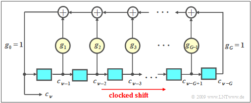
A feedback shift register can be used to generate a sequence with favorable ACF properties if the feedback coefficients $g_i$ with index $i = 1, \text{...} \ , G-1$ are chosen appropriately.
- The sequence $〈c_ν〉$ is not random in the strict sense, but periodic.
- However, due to the large period length $P$ it appears stochastic to an uninitiated observer.
- One speaks of a »pseudo–noise sequence« or "PN sequence" for short.
$\text{PN generators}$ have the following properties, see chapter "Generation of Discrete Random Variables" in the book "Theory of Stochastic Signals":
- The binary values $c_{ν-1}, \text{...} \ , c_{ν-G}$ generated at earlier times are stored in the $G$ memory cells of the shift register. We refer to $G$ as the "degree of the shift register".
- The coefficients $g_1, \ \text{...} \ , g_{G-1}$ are binary values, where a "1" indicates a feedback at the corresponding location of the shift register and a "0" indicates no feedback.
- For the currently generated symbol, with $g_i ∈ \{0, 1\}$ and $i = 1,\ \text{...}\ , G-1$:
- $$c_\nu = (g_1\cdot c_{\nu-1}+g_2\cdot c_{\nu-2}+\ \text{...}\ +g_i\cdot c_{\nu-i}+\ \text{...}\ +g_{G-1}\cdot c_{\nu-G+1}+ c_{\nu-G})\hspace{0.1cm} \rm mod \hspace{0.2cm}2.$$
- The modulo-2 addition can be realized for example by an $\rm XOR$ operation:
- $$(x + y)\hspace{0.2cm} \rm mod\hspace{0.2cm}2 = {\it x}\hspace{0.2cm}\rm XOR\hspace{0.2cm} {\it y} = \left\{ \begin{array}{*{2}{c}} 0 & \rm if\hspace{0.1cm} {\it x}= {\it y},\\ 1 & \rm if\hspace{0.1cm} {\it x}\neq {\it y}. \\ \end{array} \right.$$
- If not all $G$ memory cells are preallocated with zeros, the result is a periodic random sequence $〈c_ν〉$. The period length $P$ of this sequence depends strongly on the feedback coefficients $g_i$.
- For each degree $G$ there are at least two configurations with the maximum period $P_{\rm max} = 2^G – 1$ for this.
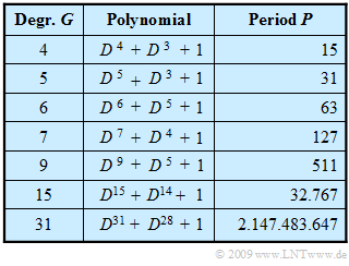
In the table on the right, for some values of $G$, the generator polynomial $G(D)$ of such an M-sequence and the corresponding (maximum) period length $P$ are given, where "M" stands for "Maximum". In the following the statements made here are clarified at the example $G = 4$.
$\text{Example 1:}$ The diagram shows two possible arrangements for generating a PN sequence of maximum length for $G = 4$ ⇒ $P = 15$.
- The octal representation of the binary number $(g_G, \ \text{...} \ ,g_2, g_1, g_0)$ is usually chosen as the abbreviation. Basically $g_0 = g_G = 1$ is to be set.
- For the left generator: $\rm (11001)_{binary} = (31)_{octal}$. The corresponding generator polynomial is:
- $$G_1(D) = D^4 + D^3 +1\hspace{0.05cm}.$$
- For the right generator: $\rm (10011)_{binary} = (23)_{octal}$. This generator can be described by the polynomial
- $$G_2(D) =D^4 + D +1 \hspace{0.05cm}.$$
- The polynomial $G_2(D)$ is reciprocal to $G_{\rm 1}(D)$:
- $$G_{\rm 2}(D) = D^4 \cdot (D^{-4} + D^{-3} +1) =D^4 + D +1 \hspace{0.05cm}.$$
Since both $G_1(D)$ and $G_{\rm 2}(D)$ are $\text{primitive generator polynomials}$ (the proof for this is not easy), both output sequences have the maximum period length $P = 15$ for $G = 4$.
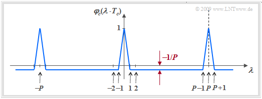
As shown in "Exercise 5.3", the PACF in unipolar representation ⇒ $c_ν ∈ \{0, 1\}$ results in
- $${\it \varphi}_{c{\rm ,\hspace{0.15cm}unipolar} }(\lambda \cdot T_c) = \left\{ \begin{array}{c}(P+1)/(2P) \\ (P+1)/(4P) \\ \end{array} \right. \begin{array}{*{10}c} \ \ {\rm{for} }\ \lambda = 0, \pm P, \pm 2P, \text{...} \hspace{0.05cm} \\ {\rm{otherwise} } \hspace{0.05cm}. \\ \end{array}$$
After conversion to bipolar coefficients $(0 \ ⇒ +1$, $1 \ ⇒ -1)$, we obtain:
- $${\it \varphi}_{c{\rm ,\hspace{0.15cm}bipolar} }(\lambda \cdot T_c) = \left\{ \begin{array}{c}1 \\ -P \\ \end{array} \right. \begin{array}{*{10}c} \ \ {\rm{for} }\ \lambda = 0, \pm P, \pm 2P, \text{...} \hspace{0.05cm} \\ {\rm{otherwise} } \hspace{0.05cm}. \\ \end{array}$$
- One can see from the bottom diagram the desired distinct PACF peaks at intervals of period $P$.
- The PCCF properties of PN sequences are less good, as will be shown in chapter "Error Probability of Direct-Sequence Spread Spectrum Modulation".
Code families with M-sequences
In CDMA, a specific spreading sequence of the same period length is required for each subscriber. A »code family« is defined as a set (as large as possible) of spreading sequences of the same period length $P$, each valid for a register level $G$.
The table shows that the number of PN sequences of maximum length is very small. For the degree $G = 5$ ⇒ $P = 31$, for example, there are just six M-sequences, namely the PN generators with the octal identifiers $(45), (51), (57), (67), (73)$ and $(75)$.
Furthermore, the term »powerfulness« of the code family can also be found in the literature.
- This quantity indicates how many M-sequences and thus simultaneous CDMA subscribers are possible if it is required that all code pairs have "favorable PCCF properties".
- For reasons of space, it cannot be explicitly stated here what exactly is meant by "favorable". For this, we refer to the original literature, for example [ZP85][1].
The last row in the above table makes it clear that the powerfulness of M-sequence code families is extremely limited, even if $G$ is large and thus the period length $P$ is large, too. If $G$ is a multiple of $4$ ⇒ $P = 15$, $P = 255$, $P = 4095$ etc., there are essentially no favorable pairs.
Gold Codes
To obtain larger code families than with M-sequences, the requirements for the periodic cross-correlation function $\rm (PCCF)$ must be weakened. With this restriction, code families with a much greater powerfulness are obtained, so that more CDMA subscribers can also be supplied.
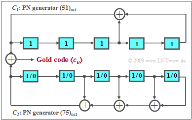
Gold codes use this principle. The rule for generating a »Gold code family« $\rm (GCF)$ is where a "+" denotes a modulo-2 addition:
- $${\rm GCF}(C_1,\ C_2) = \{ C_1,\ C_2,\ C_1 + C_2,\ C_1 + D \cdot C_2,\ C_1 + D^2 \cdot C_2, \ \text{...} \ ,\ C_1 + D^{P-1} \cdot C_2 \} \hspace{0.05cm}.$$
The principle is illustrated in the diagram by an example:
- The sequences $C_1$ and $C_2$ are a convenient pair of "M-sequences" of the same period length, for example, the PN generators with the octal identifiers $(51)$ and $(75)$ of degree $G = 5$ and thus the period length $P = 31$.
- The Gold code family consists, on the one hand, of the "M-sequences" $C_1$ and $C_2$ and of some modulo-2 additions of these sequences. $C_1$ is used with a fixed phase (characterized by the preallocation of all memory cells with ones), while all $P$ possible initial phases are permissible for the sequence $C_2$ (all preallocations except the zero allocation).
- If such a code family is used for CDMA, a total of $K_{\rm GCF} = P + 2 = 2^G + 1$ sequences are available. However, the PACF of these sequences is now no longer bivalent like the two PN sequences $(+1$ and $-1/31)$, but quadrivalent $(+1$, $+7/31$, $-1/31$, $-9/31)$. The phase of $C_2$ changes the specific progression, but not the possible PACF values.
Gold codes are used for scrambling in UMTS, for example, as explained in the chapter "Spreading codes and scrambling with UMTS" in the book "Examples of Communication Systems".
- The two master code shift registers are each constructed with $G = 18$ memory cells.
- This results in the period length $P = 262\hspace{0.05cm} 143$.
Walsh functions
Spreading sequences with very favorable PCCF properties are the so-called »Walsh functions«, whose construction is based on the »Hadamard matrix« and can be performed in a simple way by recursion. Starting from the matrix $\mathbf H_2$, further Hadamard matrices $\mathbf H_{2J}$ can be generated as follows:
- $${\mathbf{H}_{2}} = \left[ \begin{array}{ccc} +1 & +1 \\ +1 & -1 \end{array} \right] \hspace{0.5cm} \Rightarrow \hspace{0.5cm}{\mathbf{H}_{2J}} = \left[ \begin{array}{ccc} \mathbf{H}_J & \mathbf{H}_J \\ \mathbf{H}_J & -\mathbf{H}_J \end{array} \right] $$
- $$\hspace{0.5cm} \Rightarrow \hspace{0.5cm} {\mathbf{H}_{4}} = \left[ \begin{array}{cccc} +1 & +1 & +1 & +1 \\ +1 & -1 & +1 & -1 \\ +1 & +1 & -1 & -1 \\+1 & -1 & -1 & +1 \end{array} \right] .$$
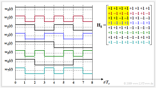
The $J$ rows of such a matrix describe the $J$ possible spreading sequences $($each of length $J)$, which are numbered $w_0(t)$ to $w_{J–1}(t)$.
The diagram shows the Hadamard matrix $\mathbf H_8$ (right) and the $J -1$ spreading sequences that can be constructed with it.
- $J - 1$ because the sequence $w_0(t)$ without spreading effect is usually not used.
- Please note the color allocation between the rows of the Hadamard matrix and the spreading sequence $w_j(t)$ in the graphic. The matrix $\mathbf H_4$ is highlighted in yellow.
- The HTML5/JavaScript applet "Generation of Walsh functions" shows the construction algorithm of such sequences.
Further applies:
- If one takes any two lines and forms the correlation (averaging over the products), the PCCF value always results in zero. Thus, Walsh functions for a distortion-free channel and a synchronous CDMA system are optimal spreading sequences due to their orthogonality.
- In contrast, for asynchronous operation (example: uplink of a mobile radio system) or de-orthogonalization due to multipath propagation, Walsh functions alone are not necessarily suitable for band spreading - see "Exercise 5.4".
- Regarding PACF (periodic ACF), these consequences are less good: Each single Walsh function has a different PACF and each single PACF is less favorable than for a comparable PN sequence. This means: Synchronization is more difficult with Walsh functions than with PN sequences.
Codes with variable spreading factor (OVSF codes)
The 3G mobile communications system $\text{UMTS}$ provides various data rates. For this purpose
- spreading sequences with different spreading factors $J = 4$ to $J = 512$ are required,
- which must all be orthogonal to each other.
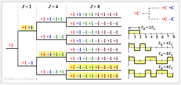
The so-called »OVSF codes« ("Orthogonal Variable Spreading Factor") can be created with the help of a code tree. Thereby two new codes $(+C \ +\hspace{-0.05cm}C)$ and $(+C \ -\hspace{-0.05cm}C)$ are created at each branching from a code $C$, as indicated in the graphic above right.
It should be noted that no predecessor and successor of a code may be used by other participants. In this example, the following selection could therefore be made (among others):
- eight codes with the spreading factor $J = 8$, or
- the four highlighted codes – once with $J = 2$, once with $J = 4$ and twice with $J = 8$.
In the second case, the other six $J = 8$ codes cannot be used because they begin with "$+1 \ +\hspace{-0.05cm}1$" or with "$+1 \ -\hspace{-0.05cm}1 \ +\hspace{-0.05cm}1 \ -\hspace{-0.05cm}1$".
From the four spreading sequences in the graphic at the bottom right, it can be seen that with a constant chip duration $T_c$, the user with spreading factor $J = 2$ can transmit at a higher data rate than the users with $J = 4$ or $J = 8$ because his bit duration $T_{\rm B}$ is smaller.
From the graph, we can further see that the periodic cross-correlation function $\rm (PCCF)$ is always zero at the point $τ = 0$.
- That means: If one forms the product of any two of these sequences and integrates over the represented time range, the value $0$ always results.
- This also means: An OVSF code is orthogonal to all other OVSF codes of the same family as long as there are no shifts.
Note: The (German language) SWF applet "OVSF codes" shows the construction algorithm of these codes and the allowed selection of spreading sequences.
Exercises for the chapter
Exercise 5.3: PACF of PN Sequences
Exercise 5.3Z: Realization of a PN Sequence
Exercise 5.4: Walsh Functions (PCCF, PACF)
References
- ↑ Ziemer, R.; Peterson, R. L.: Digital Communication and Spread Spectrum Systems. New York: McMillon, 1985.
