Difference between revisions of "Linear and Time Invariant Systems/Inverse Laplace Transform"
| (138 intermediate revisions by 9 users not shown) | |||
| Line 1: | Line 1: | ||
{{Header | {{Header | ||
| − | |Untermenü= | + | |Untermenü=Description of Causal Realizable Systems |
| − | |Vorherige Seite= | + | |Vorherige Seite=Laplace_Transform_and_p-Transfer_Function |
| − | |Nächste Seite= | + | |Nächste Seite=Some_Results_from_Transmission_Line_Theory |
}} | }} | ||
| − | == | + | ==Problem formulation and prerequisites== |
| − | + | <br> | |
| + | {{BlaueBox|TEXT= | ||
| + | $\text{Task:}$ This chapter deals with the following problem: | ||
| + | *The $p$–spectral function $Y_{\rm L}(p)$ is given in »pole-zero notation«. | ||
| + | *The »'''inverse Laplace transform'''«, i.e. the associated time function $y(t)$ is searched-for, where the following notation should hold: | ||
| + | :$$y(t) = {\rm L}^{-1}\{Y_{\rm L}(p)\}\hspace{0.05cm} , \hspace{0.3cm}{\rm briefly}\hspace{0.3cm} | ||
| + | y(t) \quad \circ\!\!-\!\!\!-^{\hspace{-0.25cm}\rm L}\!\!\!-\!\!\bullet\quad Y_{\rm L}(p)\hspace{0.05cm} .$$}} | ||
| − | [[File: | + | [[File:EN_LZI_T_3_3_S1.png |right|frame|Prerequisites for the chapter "Inverse Laplace Transform"]] |
| − | + | The graph summarizes the prerequisites for this task. | |
| − | |||
| − | |||
| + | *$H_{\rm L}(p)$ describes the transfer function of the causal system and $Y_{\rm L}(p)$ specifies the Laplace transform of the output signal $y(t)$ considering the input signal $x(t)$ . $Y_{\rm L}(p)$ is characterized by $N$ poles, by $Z ≤ N$ zeros and by the constant $K.$ | ||
| + | |||
| + | *Poles and zeros exhibit the properties mentioned in the [[Linear_and_Time_Invariant_Systems/Laplace_Transform_and_p-Transfer_Function#Properties_of_poles_and_zeros|»last chapter«]]: Poles are only allowed in the left $p$–half plane or on the imaginary axis; zeros are also allowed in the right $p$–half plane. | ||
| + | |||
| + | *All »singularities« – this is the generic term for poles and zeros – are either real or exist as pairs of conjugate-complex singularities. Multiple poles and zeros are also allowed. | ||
| + | |||
| + | *With the input $x(t) = δ(t)$ ⇒ $X_{\rm L}(p) = 1$ ⇒ $Y_{\rm L}(p) = H_{\rm L}(p)$, the output signal $y(t)$ then describes the [[Linear_and_Time_Invariant_Systems/System_Description_in_Time_Domain#Impulse_response|»impulse response«]] $h(t)$ of the transmission system. For this purpose, only the singularities drawn in green in the graph may be used for computation. | ||
| − | + | *A unit jump function $x(t) = γ(t)$ ⇒ $ X_{\rm L} = 1/p$ at the input causes the output signal $y(t)$ to be equal to the [[Linear_and_Time_Invariant_Systems/System_Description_in_Time_Domain#Step_response|»step response«]] $σ(t)$ of $H_{\rm L}(p)$ . In addition to the singularities of $H_{\rm L}(p)$, the pole $($shown in red in the graph$)$ at $p = 0$ must now also be taken into account for computation. | |
| − | * | + | |
| − | * | + | *Possible as input $x(t)$ are only signals for which $X_{ \rm L}(p)$ can be expressed in pole-zero notation (see the [[Linear_and_Time_Invariant_Systems/Laplace_Transform_and_p-Transfer_Function#Some_important_Laplace_correspondences|$\text{table}$]] in the chapter »Laplace Transform and $p$–Transfer Function»$)$, for example a cosine or sine signal switched on at time $t = 0$ . |
| − | * | + | |
| − | + | *So, a rectangular signal $x(t)\ \ ⇒ \ \ X_{\rm L}(p) = (1 - {\rm e}^{\hspace{0.05cm}p\hspace{0.05cm}\cdot \hspace{0.05cm} T})/p$ is not possible in the approach described here. However, the rectangular response $y(t)$ can be computed indirectly as the difference of two step responses. | |
| − | == | + | ==Some results of function theory== |
| − | + | <br> | |
| − | + | In contrast to the [[Signal_Representation/Fourier_Transform_and_Its_Inverse#The_first_Fourier_integral|»Fourier integrals«]], which differ only slightly in the two directions of transformation, for »Laplace« the computation of $y(t)$ from $Y_{\rm L}(p)$ – that is the inverse transformation – is | |
| − | + | *much more difficult than computing $Y_{\rm L}(p)$ from $y(t)$, | |
| − | + | ||
| − | + | *unresolvable or solvable only very laboriously by elementary means. | |
| − | $ | ||
| − | |||
| − | |||
| + | {{BlaueBox|TEXT= | ||
| + | $\text{Definition:}$ | ||
| + | In general, the following holds for the »'''inverse Laplace transform'''«: | ||
| + | :$$y(t) = {\rm L}^{-1}\{Y_{\rm L}(p)\}= \lim_{\beta \hspace{0.05cm}\rightarrow \hspace{0.05cm}\infty} \hspace{0.15cm} \frac{1}{ {\rm j} \cdot 2 \pi}\cdot \int_{ \alpha - {\rm j} \hspace{0.05cm}\cdot \hspace{0.05cm}2 \pi \beta } ^{\alpha+{\rm j} \hspace{0.05cm}\cdot \hspace{0.05cm}2 \pi \beta} Y_{\rm L}(p) \hspace{0.05cm}\cdot \hspace{0.05cm} {\rm e}^{\hspace{0.05cm}p \hspace{0.05cm}\cdot \hspace{0.05cm} t}\hspace{0.1cm}{\rm | ||
| + | d}p \hspace{0.05cm} .$$ | ||
| + | #The integration is parallel to the imaginary axis. | ||
| + | #The real part $α$ is to be chosen such that all poles are located to the left of the integration path.}} | ||
| + | The left graph illustrates this line integral along the red dotted vertical ${\rm Re}\{p\}= α$. This integral is solvable using [https://en.wikipedia.org/wiki/Jordan%27s_lemma »Jordan's lemma of complex analysis«]. In this tutorial only a very short and simple summary of the approach is depicted: | ||
| + | [[File:EN_LZI_T_3_3_S2.png |right|frame|Line integral together with left and right circular integral]] | ||
| + | |||
| + | #The line integral can be divided into two circular integrals so that all poles are located in the left circular integral while the right circular integral may only contain zeros. | ||
| + | #According to the theory of functions, the right circular integral yields the time function $y(t)$ for negative times. | ||
| + | #Due to causality, $y(t < 0)$ must be identical to zero, but according to the fundamentals of function theorem this is only true if there are no poles in the right $p$–half-plane. | ||
| + | #In contrast, the integral over the left semicircle yields the time function for $t ≥ 0$. | ||
| + | #This encloses all poles and can be computed using the »'''residue theorem'''« in a $($relatively$)$ simple way, as it will be shown in the next sections. | ||
| + | <br clear=all> | ||
| + | ==Formulation of the residue theorem== | ||
| + | <br> | ||
| + | It is further assumed that the transfer function $Y_{\rm L}(p)$ can be expressed in pole-zero notation by | ||
| + | *the constant factor $K$, | ||
| + | *the $Z$ »zeros« $p_{{\rm o}i}$ $(i = 1$, ... , $Z)$ and | ||
| + | *the $N$ »poles« $p_{{\rm x}i}$ $(i = 1$, ... , $N$). | ||
| + | We also assume $Z < N$. The number of »distinguishable poles« is denoted by $I$. Multiple poles are counted only once to determine $I$. Thus, the following holds for the [[Linear_and_Time_Invariant_Systems/Inverse_Laplace_Transform#Some_results_of_function_theory|$\text{sketch}$]] in the last section considering the double pole: | ||
| + | :$$N = 5,\hspace{0.3cm} I = 4.$$ | ||
| + | {{BlaueBox|TEXT= | ||
| + | $\text{Residue Theorem:}$ | ||
| + | Considering the above conditions, the »'''inverse Laplace transform'''« of $Y_{\rm L}(p)$ for times $t ≥ 0$ is obtained as the sum of $I$ natural oscillations of the poles, which are called the »residuals« – abbreviated as $\rm Res$: | ||
| + | :$$y(t) = \sum_{i=1}^{I}{\rm Res} \bigg \vert _{p \hspace{0.05cm}= \hspace{0.05cm}p_{{\rm x}_i}} \hspace{-0.7cm}\{Y_{\rm L}(p)\cdot {\rm e}^{p \hspace{0.05cm}t}\} \hspace{0.05cm} .$$ | ||
| + | Since $Y_{\rm L}(p)$ is only specifiable for causal signals, $y(t < 0) = 0$ always holds for negative times. | ||
| + | |||
| + | *In general, the following holds for a pole of multiplicity $l$ : | ||
| + | :$${\rm Res} \bigg \vert _{p \hspace{0.05cm}= \hspace{0.05cm}p_{ {\rm x}_i} } \hspace{-0.7cm}\{Y_{\rm L}(p)\cdot {\rm e}^{p t}\}= \frac{1}{(l-1)!}\cdot \frac{ {\rm d}^{\hspace{0.05cm}l-1} }{ {\rm d}p^{\hspace{0.05cm}l-1} }\hspace{0.15cm} \left \{Y_{\rm L}(p)\cdot (p - p_{ {\rm x}_i})^{\hspace{0.05cm}l}\cdot {\rm e}^{p \hspace{0.05cm}t}\right\} \bigg \vert_{p \hspace{0.05cm}= \hspace{0.05cm}p_{ {\rm x}_i} } \hspace{0.05cm} .$$ | ||
| + | *The following is obtained out of it with $l = 1$ for a simple pole as a special case: | ||
| + | :$${\rm Res} \bigg\vert_{p \hspace{0.05cm}= \hspace{0.05cm}p_{ {\rm x}_i} } \hspace{-0.7cm}\{Y_{\rm L}(p)\cdot {\rm e}^{p t}\}= Y_{\rm L}(p)\cdot (p - p_{ {\rm x}_i} )\cdot {\rm e}^{p \hspace{0.05cm}t} \bigg \vert _{p \hspace{0.05cm}= \hspace{0.05cm}p_{ {\rm x}_i} } \hspace{0.05cm} .$$}} | ||
| + | |||
| + | |||
| + | In the next sections, the »residue theorem« is illustrated by three detailed examples corresponding to the three constellations in [[Linear_and_Time_Invariant_Systems/Laplace_Transform_and_p-Transfer_Function#Properties_of_poles_and_zeros|$\text{Example 3}$]] of chapter »Laplace transform and p-transfer function«: | ||
| + | *So, we consider again the two-port network with an inductance $L = 25 \ \rm µH$ in the longitudinal branch as well as the the series connection of an ohmic resistance $R = 50 \ \rm Ω$ and a capacitance $C$ in the transverse branch. | ||
| + | |||
| + | *For the latter, we consider three different values, namely $C = 62.5 \ \rm nF$, $C = 8 \ \rm nF$ and $C = 40 \ \rm nF$. | ||
| + | |||
| + | *The following is always assumed: $x(t) = δ(t) \; ⇒ \; X_{\rm L}(p) = 1$ ⇒ $Y_{\rm L}(p) = H_{\rm L}(p)$ ⇒ the output signal $y(t)$ is equal to the impulse response $h(t)$. | ||
| + | |||
| + | ==Aperiodically decaying impulse response== | ||
| + | <br> | ||
| + | The following is obtained for the $p$–transfer function computed in the section [[Linear_and_Time_Invariant_Systems/Laplace_Transform_and_p-Transfer_Function#Pole-zero_representation_of_circuits|»pole-zero representation of circuits«]] with the capacitance $C = 62.5 \ \rm nF$. The other numerical values are given in the graph below: | ||
| + | [[File: EN_LZI_T_3_3_S3a.png|right|frame|Aperiodically decaying impulse response]] | ||
| + | |||
| + | :$$H_{\rm L}(p)= K \cdot \frac {p - p_{\rm o }} {(p - p_{\rm x 1})(p - p_{\rm x 2})}= 2 \cdot \frac {p + 0.32 } | ||
| + | {(p +0.4)(p +1.6 )} \hspace{0.05cm} .$$ | ||
| + | |||
| + | Note the normalization of $p$, $K$ and also of all poles and zeros by the factor ${\rm 10^6} · 1/\rm s$. | ||
| + | |||
| + | ⇒ The impulse response is composed of $I = N = 2$ natural oscillations. For $t < 0$, these are equal to zero. | ||
| + | *The residual of the pole at $p_{{\rm x}1} =\ –0.4$ yields the following time function: | ||
| + | :$$h_1(t) = {\rm Res} \bigg |_{p \hspace{0.05cm}= \hspace{0.05cm}p_{{\rm x}1}} \hspace{-0.7cm}\{H_{\rm L}(p)\cdot {\rm e}^{p t}\}= H_{\rm L}(p)\cdot (p - p_{{\rm x}1})\cdot {\rm e}^{p \hspace{0.05cm}t} \bigg |_{p \hspace{0.05cm}= \hspace{0.05cm}p_{{\rm x}1}}$$ | ||
| + | : $$\Rightarrow \hspace{0.3cm}h_1(t) = 2 \cdot \frac {p + 0.32 } {p +0.4}\cdot {\rm e}^{p \hspace{0.05cm}t} \bigg |_{p \hspace{0.05cm}= \hspace{0.05cm}-0.4}= - \frac {2 } {15}\cdot {\rm e}^{-0.4 \hspace{0.05cm} t} \hspace{0.05cm}. $$ | ||
| + | *In the same way, the residual of the second pole at $p_{{\rm x}2} = \ –1.6$ can be computed: | ||
| + | :$$h_2(t) = {\rm Res} \bigg |_{p \hspace{0.05cm}= \hspace{0.05cm}p_{{\rm x}2}} \hspace{-0.7cm}\{H_{\rm L}(p)\cdot {\rm e}^{p t}\}= H_{\rm L}(p)\cdot (p - p_{{\rm x}2})\cdot {\rm e}^{p \hspace{0.05cm}t} \bigg |_{p \hspace{0.05cm}= \hspace{0.05cm}p_{{\rm x}2}}$$ | ||
| + | :$$\Rightarrow \hspace{0.3cm}h_2(t) = 2 \cdot \frac {p + 0.32 } {p +1.6}\cdot {\rm e}^{p \hspace{0.05cm}t} \bigg |_{p \hspace{0.05cm}= \hspace{0.05cm}-1.6}= \frac {32 } {15}\cdot {\rm e}^{-1.6 \hspace{0.05cm} t} \hspace{0.05cm}. $$ | ||
| + | |||
| + | The graph shows $h_1(t)$ and $h_2(t)$ as well as the sum signal $h(t)$. | ||
| + | #The normalization factor $1/T = 10^6 · \rm 1/s$ is taken into account here so that the time is normalized to $T = 1 \ \rm µ s$ . | ||
| + | #For $t =0$, $T \cdot h(t=0) = {32 }/ {15} -{2 }/ {15}= 2 \hspace{0.05cm}$ is obtained as a result. | ||
| + | #For times $t > 2 \ \rm µ s$, the impulse response is negative $($although only slightly and difficult to see in the graph$)$. | ||
| + | |||
| + | |||
| + | ==Attenuated-oscillatory impulse response== | ||
| + | <br> | ||
| + | The component values $R = 50 \ \rm Ω$, $L = 25 \ \rm µ H$ and $C = 8 \ \rm nF$ result in two conjugate complex poles at $p_{{\rm x}1} = \ –1 + {\rm j} · 2$ and $p_{{\rm x}2} = \ –1 - {\rm j} · 2$. | ||
| + | [[File:EN_LZI_T_3_3_S3b.png|right|frame| Attenuated-oscillatory impulse response]] | ||
| + | |||
| + | *The zero is located at $p_{\rm o} = \ –2.5$. | ||
| + | |||
| + | *$K = 2$ holds | ||
| + | |||
| + | *All numerical values are to be multiplied by factor $1/T$ $(T = 1\ \rm µ s$). | ||
| + | |||
| + | |||
| + | Applying the residue theorem to this configuration then it is obtained: | ||
| + | |||
| + | :$$h_1(t) = K \cdot \frac {p_{\rm x 1} - p_{\rm o }} {p_{\rm x 1} - p_{\rm x 2}} \cdot {\rm e}^{\hspace{0.05cm}p_{\rm x 1} \cdot \hspace{0.05cm}t} $$ | ||
| + | :$$\Rightarrow \hspace{0.3cm}h_1(t) = 2 \cdot \frac {-1 + {\rm j}\cdot 2 +2.5} {(-1 + {\rm j}\cdot 2) - (-1 - {\rm j}\cdot 2)}\cdot {\rm e}^{\hspace{0.05cm}p_{\rm x 1} | ||
| + | \cdot\hspace{0.05cm}t}$$ | ||
| + | :$$\Rightarrow \hspace{0.3cm}h_1(t) = 2 \cdot \frac {1.5 + {\rm j}\cdot 2} {{\rm j}\cdot 4}\cdot {\rm e}^{\hspace{0.05cm}p_{\rm x 1} \cdot\hspace{0.05cm}t}= (1 - {\rm j}\cdot 0.75)\cdot {\rm | ||
| + | e}^{-t}\cdot {\rm e}^{\hspace{0.03cm}{\rm j}\hspace{0.05cm}\cdot \hspace{0.05cm} 2t} \hspace{0.05cm} ,$$ | ||
| + | |||
| + | :$$ h_2(t) = K \cdot \frac {p_{\rm x 2} - p_{\rm o }} {p_{\rm x 2} - p_{\rm x 1}}\cdot {\rm e}^{\hspace{0.05cm}p_{\rm x 2} \hspace{0.03cm}\cdot \hspace{0.05cm}t} $$ | ||
| + | :$$\Rightarrow \hspace{0.3cm} h_2(t) = 2 \cdot \frac {-1 - {\rm j}\cdot 2 +2.5} {(-1 - {\rm j}\cdot 2) - (-1 + {\rm j}\cdot 2)}\cdot {\rm e}^{\hspace{0.05cm}p_{\rm x 2} \hspace{0.03cm}\cdot\hspace{0.05cm}t} $$ | ||
| + | :$$\Rightarrow \hspace{0.3cm}h_2(t) =2 \cdot \frac {1.5 - {\rm j}\cdot 2} {-{\rm j}\cdot 4}\cdot {\rm e}^{\hspace{0.05cm}p_{\rm x 2} \hspace{0.03cm}\cdot\hspace{0.05cm}t}= (1 + {\rm j}\cdot 0.75)\cdot {\rm e}^{-t}\cdot {\rm e}^{\hspace{0.03cm}-{\rm j}\hspace{0.05cm}\cdot \hspace{0.05cm} 2t} \hspace{0.05cm} . $$ | ||
| + | |||
| + | Using [[Signal_Representation/Calculating_With_Complex_Numbers#Representation_by_magnitude_and_phase|»Euler's theorem«]] the following is obtained for the sum signal: | ||
| + | :$$h(t) = h_1(t) + h_2(t)\hspace{0.3cm} | ||
| + | \Rightarrow \hspace{0.3cm}h(t) = {\rm e}^{-t}\cdot \big [ (1 - {\rm j}\cdot 0.75)\cdot (\cos() + {\rm j}\cdot \sin())+ | ||
| + | + (1 + {\rm j}\cdot 0.75)\cdot (\cos() - {\rm j}\cdot \sin())\big ]$$ | ||
| + | :$$\Rightarrow \hspace{0.3cm}h(t) ={\rm e}^{-t}\cdot \big [ 2\cdot \cos(2t) + 1.5 \cdot \sin(2t)\big ]\hspace{0.05cm} . $$ | ||
| + | |||
| + | The graph shows the attenuated-oscillatory impulse response $h(t)$ attenuated by ${\rm e}^{–t}$ for this pole–zero configuration. | ||
| + | |||
| + | |||
| + | ==Critically attenuated case== | ||
| + | <br> | ||
| + | With $R = 50 \ \rm Ω$, $L = 25 \ \rm µ H$ and $C = 40 \ \rm nF$ we get the so-called »critically attenuated case«: | ||
| + | :$$H_{\rm L}(p)= K \cdot \frac {p - p_{\rm o }} {(p - p_{\rm x })^2}= 2 \cdot \frac {p + 0.5 } {(p +1)^2} \hspace{0.05cm} .$$ | ||
| + | |||
| + | The capacitance $C = 40 \ \rm nF$ is the smallest possible value for which there are just real pole places. These coincide, that $p_{\rm x} = \ -1$ is a double pole place. The time function is thus according to the residue theorem with $l = 2$: | ||
| + | :$$h(t) = {\rm Res} \bigg |_{p \hspace{0.05cm}= \hspace{0.05cm}p_{ {\rm x} } } \hspace{-0.7cm}\{H_{\rm L}(p)\cdot {\rm e}^{p t}\}= \frac{ {\rm d} }{ {\rm d}p}\hspace{0.15cm} | ||
| + | \left \{H_{\rm L}(p)\cdot (p - p_{ {\rm x} })^2\cdot {\rm e}^{p \hspace{0.05cm}t}\right\} \bigg |_{p \hspace{0.05cm}= \hspace{0.05cm}p_{ {\rm x} } } = K \cdot \frac{ {\rm d} }{ {\rm d}p}\hspace{0.15cm}\left \{ (p - p_{ {\rm o} })\cdot {\rm e}^{p \hspace{0.05cm}t}\right\} \bigg |_{p \hspace{0.05cm}= \hspace{0.05cm}p_{ {\rm x} } } \hspace{0.05cm} .$$ | ||
| + | |||
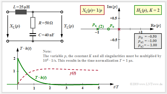
| + | [[File:EN_LZI_T_3_3_S3c.png |right|frame| Impulse response and step response of the critically attenuated case]] | ||
| + | Using the »product rule« of differential calculus, this gives: | ||
| + | :$$h(t) = K \cdot \left [ {\rm e}^{p \hspace{0.05cm}t} + (p - p_{ {\rm o} })\cdot t \cdot {\rm e}^{p \hspace{0.05cm}t} \right ] \bigg |_{p \hspace{0.05cm}= \hspace{0.05cm}-1} = {\rm e}^{-t}\cdot \left ( 2 - t \right) | ||
| + | \hspace{0.05cm} .$$ | ||
| + | |||
| + | The graph shows this impulse response $($green curve$)$ in normalized representation. It differs only slightly from the one with two different poles at $-0.4$ and $-1.6$ . | ||
| + | |||
| + | The signal drawn in red ⇒ $y(t) = 1 - {\rm e}^{-t} + t \cdot {\rm e}^{-t}$ results when a step function $\gamma(t)$ is considered at the input ⇒ »step response«. | ||
| + | |||
| + | To calculate the step response $\sigma(t) = y(t)$ one can alternatively | ||
| + | *consider the additional red pole at $p = 0$ in the residual calculation, | ||
| + | |||
| + | *or form the integral over the impulse response $h(t)$. | ||
| + | |||
| + | |||
| + | ==Partial fraction decomposition== | ||
| + | <br> | ||
| + | Prerequisite for the application of the residue theorem is that there are less zeros than poles ⇒ $Z$ must always be smaller than $N$ . | ||
| + | |||
| + | *If, on the other hand, as in the case of a high-pass filter $Z = N$, then the limit of the p–transfer function $H_{\rm L}(p)$ for large $p$ is not equal to zero, | ||
| + | |||
| + | *If the associated time signal $y(t)$ also contains [[Signal_Representation/Direct_Current_Signal_-_Limit_Case_of_a_Periodic_Signal#Dirac_.28delta.29_function_in_frequency_domain|»Dirac delta functions«]], the residue theorem fails and a [https://en.wikipedia.org/wiki/Partial_fraction_decomposition »'''partial fraction decomposition'''«] must be performed. | ||
| + | |||
| + | |||
| + | The procedure is to be clarified exemplarily for a high-pass of first order. | ||
| + | |||
| + | {{GraueBox|TEXT= | ||
| + | $\text{Example 1:}$ | ||
| + | The $p$-transfer function of a »first-order RC high-pass filter« can be transformed by splitting off a constant as follows: | ||
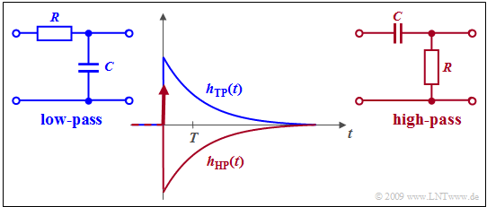
| + | [[File:EN_LZI_T_3_3_S5_v2.png |right|frame| Impulse response of low-pass $($blue$)$ and high-pass $($red$)$]] | ||
| + | :$$\frac{p}{p + RC} = 1- \frac{RC}{p + RC}\hspace{0.05cm} .$$ | ||
| + | Thus, the high-pass impulse response is: | ||
| + | :$$h_{\rm HP}(t) = \delta(t) - h_{\rm TP}(t) \hspace{0.05cm} .$$ | ||
| + | |||
| + | The graph shows | ||
| + | *as blue curve the impulse response $h_{\rm TP}(t)$ of the equivalent low-pass, | ||
| + | |||
| + | *as red curve the high–pass impulse response $h_{\rm HP}(t)$. | ||
| + | |||
| + | |||
| + | ⇒ The Dirac delta function is the Laplace transform of the constant value $1$, <br>while the second function to be subtracted gives the impulse response of the equivalent low-pass filter, which is given by the residue theorem with | ||
| + | :$$Z = 0,\hspace{0.2cm} N =1,\hspace{0.2cm} K = RC.$$ }} | ||
| + | |||
| + | |||
| + | |||
| + | ==Exercises for the chapter== | ||
| + | |||
| + | [[Aufgaben:Exercise_3.5:_Circuit_with_R,_L_and_C|Exercise 3.5: Circuit with R, L and C]] | ||
| + | |||
| + | [[Aufgaben:Exercise_3.5Z:_Application_of_the_Residue_Theorem|Exercise 3.5Z: Application of the Residue Theorem]] | ||
| + | |||
| + | [[Aufgaben:Exercise_3.6:_Transient_Behavior|Exercise 3.6: Transient Behavior]] | ||
| + | |||
| + | [[Aufgaben:Exercise_3.6Z:_Two_Imaginary_Poles|Exercise 3.6Z: Two Imaginary Poles]] | ||
| + | |||
| + | [[Aufgaben:Exercise_3.7:_Impulse_Response_of_a_High-Pass_Filter|Exercise 3.7: Impulse Response of a High-Pass Filter]] | ||
| + | |||
| + | [[Aufgaben:Exercise_3.7Z:_Partial_Fraction_Decomposition|Exercise 3.7Z: Partial Fraction Decomposition]] | ||
{{Display}} | {{Display}} | ||
Latest revision as of 17:03, 21 November 2023
Contents
Problem formulation and prerequisites
$\text{Task:}$ This chapter deals with the following problem:
- The $p$–spectral function $Y_{\rm L}(p)$ is given in »pole-zero notation«.
- The »inverse Laplace transform«, i.e. the associated time function $y(t)$ is searched-for, where the following notation should hold:
- $$y(t) = {\rm L}^{-1}\{Y_{\rm L}(p)\}\hspace{0.05cm} , \hspace{0.3cm}{\rm briefly}\hspace{0.3cm} y(t) \quad \circ\!\!-\!\!\!-^{\hspace{-0.25cm}\rm L}\!\!\!-\!\!\bullet\quad Y_{\rm L}(p)\hspace{0.05cm} .$$
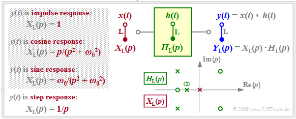
The graph summarizes the prerequisites for this task.
- $H_{\rm L}(p)$ describes the transfer function of the causal system and $Y_{\rm L}(p)$ specifies the Laplace transform of the output signal $y(t)$ considering the input signal $x(t)$ . $Y_{\rm L}(p)$ is characterized by $N$ poles, by $Z ≤ N$ zeros and by the constant $K.$
- Poles and zeros exhibit the properties mentioned in the »last chapter«: Poles are only allowed in the left $p$–half plane or on the imaginary axis; zeros are also allowed in the right $p$–half plane.
- All »singularities« – this is the generic term for poles and zeros – are either real or exist as pairs of conjugate-complex singularities. Multiple poles and zeros are also allowed.
- With the input $x(t) = δ(t)$ ⇒ $X_{\rm L}(p) = 1$ ⇒ $Y_{\rm L}(p) = H_{\rm L}(p)$, the output signal $y(t)$ then describes the »impulse response« $h(t)$ of the transmission system. For this purpose, only the singularities drawn in green in the graph may be used for computation.
- A unit jump function $x(t) = γ(t)$ ⇒ $ X_{\rm L} = 1/p$ at the input causes the output signal $y(t)$ to be equal to the »step response« $σ(t)$ of $H_{\rm L}(p)$ . In addition to the singularities of $H_{\rm L}(p)$, the pole $($shown in red in the graph$)$ at $p = 0$ must now also be taken into account for computation.
- Possible as input $x(t)$ are only signals for which $X_{ \rm L}(p)$ can be expressed in pole-zero notation (see the $\text{table}$ in the chapter »Laplace Transform and $p$–Transfer Function»$)$, for example a cosine or sine signal switched on at time $t = 0$ .
- So, a rectangular signal $x(t)\ \ ⇒ \ \ X_{\rm L}(p) = (1 - {\rm e}^{\hspace{0.05cm}p\hspace{0.05cm}\cdot \hspace{0.05cm} T})/p$ is not possible in the approach described here. However, the rectangular response $y(t)$ can be computed indirectly as the difference of two step responses.
Some results of function theory
In contrast to the »Fourier integrals«, which differ only slightly in the two directions of transformation, for »Laplace« the computation of $y(t)$ from $Y_{\rm L}(p)$ – that is the inverse transformation – is
- much more difficult than computing $Y_{\rm L}(p)$ from $y(t)$,
- unresolvable or solvable only very laboriously by elementary means.
$\text{Definition:}$ In general, the following holds for the »inverse Laplace transform«:
- $$y(t) = {\rm L}^{-1}\{Y_{\rm L}(p)\}= \lim_{\beta \hspace{0.05cm}\rightarrow \hspace{0.05cm}\infty} \hspace{0.15cm} \frac{1}{ {\rm j} \cdot 2 \pi}\cdot \int_{ \alpha - {\rm j} \hspace{0.05cm}\cdot \hspace{0.05cm}2 \pi \beta } ^{\alpha+{\rm j} \hspace{0.05cm}\cdot \hspace{0.05cm}2 \pi \beta} Y_{\rm L}(p) \hspace{0.05cm}\cdot \hspace{0.05cm} {\rm e}^{\hspace{0.05cm}p \hspace{0.05cm}\cdot \hspace{0.05cm} t}\hspace{0.1cm}{\rm d}p \hspace{0.05cm} .$$
- The integration is parallel to the imaginary axis.
- The real part $α$ is to be chosen such that all poles are located to the left of the integration path.
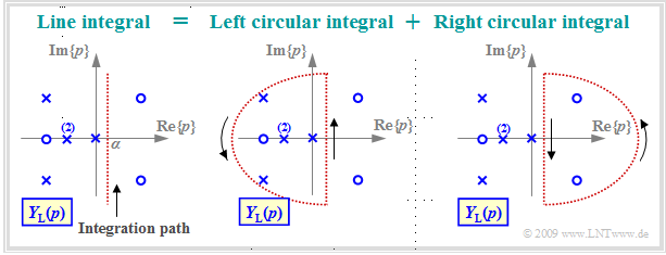
The left graph illustrates this line integral along the red dotted vertical ${\rm Re}\{p\}= α$. This integral is solvable using »Jordan's lemma of complex analysis«. In this tutorial only a very short and simple summary of the approach is depicted:
- The line integral can be divided into two circular integrals so that all poles are located in the left circular integral while the right circular integral may only contain zeros.
- According to the theory of functions, the right circular integral yields the time function $y(t)$ for negative times.
- Due to causality, $y(t < 0)$ must be identical to zero, but according to the fundamentals of function theorem this is only true if there are no poles in the right $p$–half-plane.
- In contrast, the integral over the left semicircle yields the time function for $t ≥ 0$.
- This encloses all poles and can be computed using the »residue theorem« in a $($relatively$)$ simple way, as it will be shown in the next sections.
Formulation of the residue theorem
It is further assumed that the transfer function $Y_{\rm L}(p)$ can be expressed in pole-zero notation by
- the constant factor $K$,
- the $Z$ »zeros« $p_{{\rm o}i}$ $(i = 1$, ... , $Z)$ and
- the $N$ »poles« $p_{{\rm x}i}$ $(i = 1$, ... , $N$).
We also assume $Z < N$. The number of »distinguishable poles« is denoted by $I$. Multiple poles are counted only once to determine $I$. Thus, the following holds for the $\text{sketch}$ in the last section considering the double pole:
- $$N = 5,\hspace{0.3cm} I = 4.$$
$\text{Residue Theorem:}$ Considering the above conditions, the »inverse Laplace transform« of $Y_{\rm L}(p)$ for times $t ≥ 0$ is obtained as the sum of $I$ natural oscillations of the poles, which are called the »residuals« – abbreviated as $\rm Res$:
- $$y(t) = \sum_{i=1}^{I}{\rm Res} \bigg \vert _{p \hspace{0.05cm}= \hspace{0.05cm}p_{{\rm x}_i}} \hspace{-0.7cm}\{Y_{\rm L}(p)\cdot {\rm e}^{p \hspace{0.05cm}t}\} \hspace{0.05cm} .$$
Since $Y_{\rm L}(p)$ is only specifiable for causal signals, $y(t < 0) = 0$ always holds for negative times.
- In general, the following holds for a pole of multiplicity $l$ :
- $${\rm Res} \bigg \vert _{p \hspace{0.05cm}= \hspace{0.05cm}p_{ {\rm x}_i} } \hspace{-0.7cm}\{Y_{\rm L}(p)\cdot {\rm e}^{p t}\}= \frac{1}{(l-1)!}\cdot \frac{ {\rm d}^{\hspace{0.05cm}l-1} }{ {\rm d}p^{\hspace{0.05cm}l-1} }\hspace{0.15cm} \left \{Y_{\rm L}(p)\cdot (p - p_{ {\rm x}_i})^{\hspace{0.05cm}l}\cdot {\rm e}^{p \hspace{0.05cm}t}\right\} \bigg \vert_{p \hspace{0.05cm}= \hspace{0.05cm}p_{ {\rm x}_i} } \hspace{0.05cm} .$$
- The following is obtained out of it with $l = 1$ for a simple pole as a special case:
- $${\rm Res} \bigg\vert_{p \hspace{0.05cm}= \hspace{0.05cm}p_{ {\rm x}_i} } \hspace{-0.7cm}\{Y_{\rm L}(p)\cdot {\rm e}^{p t}\}= Y_{\rm L}(p)\cdot (p - p_{ {\rm x}_i} )\cdot {\rm e}^{p \hspace{0.05cm}t} \bigg \vert _{p \hspace{0.05cm}= \hspace{0.05cm}p_{ {\rm x}_i} } \hspace{0.05cm} .$$
In the next sections, the »residue theorem« is illustrated by three detailed examples corresponding to the three constellations in $\text{Example 3}$ of chapter »Laplace transform and p-transfer function«:
- So, we consider again the two-port network with an inductance $L = 25 \ \rm µH$ in the longitudinal branch as well as the the series connection of an ohmic resistance $R = 50 \ \rm Ω$ and a capacitance $C$ in the transverse branch.
- For the latter, we consider three different values, namely $C = 62.5 \ \rm nF$, $C = 8 \ \rm nF$ and $C = 40 \ \rm nF$.
- The following is always assumed: $x(t) = δ(t) \; ⇒ \; X_{\rm L}(p) = 1$ ⇒ $Y_{\rm L}(p) = H_{\rm L}(p)$ ⇒ the output signal $y(t)$ is equal to the impulse response $h(t)$.
Aperiodically decaying impulse response
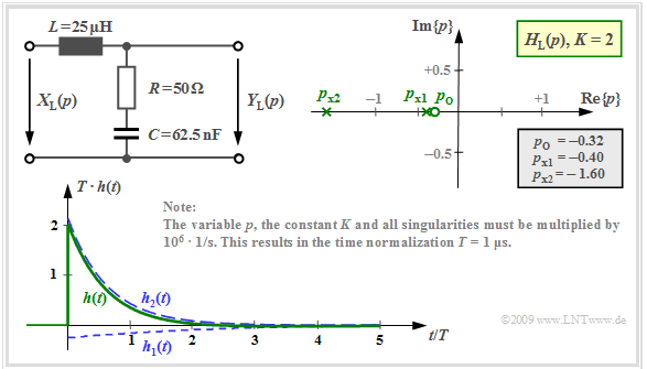
The following is obtained for the $p$–transfer function computed in the section »pole-zero representation of circuits« with the capacitance $C = 62.5 \ \rm nF$. The other numerical values are given in the graph below:
- $$H_{\rm L}(p)= K \cdot \frac {p - p_{\rm o }} {(p - p_{\rm x 1})(p - p_{\rm x 2})}= 2 \cdot \frac {p + 0.32 } {(p +0.4)(p +1.6 )} \hspace{0.05cm} .$$
Note the normalization of $p$, $K$ and also of all poles and zeros by the factor ${\rm 10^6} · 1/\rm s$.
⇒ The impulse response is composed of $I = N = 2$ natural oscillations. For $t < 0$, these are equal to zero.
- The residual of the pole at $p_{{\rm x}1} =\ –0.4$ yields the following time function:
- $$h_1(t) = {\rm Res} \bigg |_{p \hspace{0.05cm}= \hspace{0.05cm}p_{{\rm x}1}} \hspace{-0.7cm}\{H_{\rm L}(p)\cdot {\rm e}^{p t}\}= H_{\rm L}(p)\cdot (p - p_{{\rm x}1})\cdot {\rm e}^{p \hspace{0.05cm}t} \bigg |_{p \hspace{0.05cm}= \hspace{0.05cm}p_{{\rm x}1}}$$
- $$\Rightarrow \hspace{0.3cm}h_1(t) = 2 \cdot \frac {p + 0.32 } {p +0.4}\cdot {\rm e}^{p \hspace{0.05cm}t} \bigg |_{p \hspace{0.05cm}= \hspace{0.05cm}-0.4}= - \frac {2 } {15}\cdot {\rm e}^{-0.4 \hspace{0.05cm} t} \hspace{0.05cm}. $$
- In the same way, the residual of the second pole at $p_{{\rm x}2} = \ –1.6$ can be computed:
- $$h_2(t) = {\rm Res} \bigg |_{p \hspace{0.05cm}= \hspace{0.05cm}p_{{\rm x}2}} \hspace{-0.7cm}\{H_{\rm L}(p)\cdot {\rm e}^{p t}\}= H_{\rm L}(p)\cdot (p - p_{{\rm x}2})\cdot {\rm e}^{p \hspace{0.05cm}t} \bigg |_{p \hspace{0.05cm}= \hspace{0.05cm}p_{{\rm x}2}}$$
- $$\Rightarrow \hspace{0.3cm}h_2(t) = 2 \cdot \frac {p + 0.32 } {p +1.6}\cdot {\rm e}^{p \hspace{0.05cm}t} \bigg |_{p \hspace{0.05cm}= \hspace{0.05cm}-1.6}= \frac {32 } {15}\cdot {\rm e}^{-1.6 \hspace{0.05cm} t} \hspace{0.05cm}. $$
The graph shows $h_1(t)$ and $h_2(t)$ as well as the sum signal $h(t)$.
- The normalization factor $1/T = 10^6 · \rm 1/s$ is taken into account here so that the time is normalized to $T = 1 \ \rm µ s$ .
- For $t =0$, $T \cdot h(t=0) = {32 }/ {15} -{2 }/ {15}= 2 \hspace{0.05cm}$ is obtained as a result.
- For times $t > 2 \ \rm µ s$, the impulse response is negative $($although only slightly and difficult to see in the graph$)$.
Attenuated-oscillatory impulse response
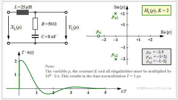
The component values $R = 50 \ \rm Ω$, $L = 25 \ \rm µ H$ and $C = 8 \ \rm nF$ result in two conjugate complex poles at $p_{{\rm x}1} = \ –1 + {\rm j} · 2$ and $p_{{\rm x}2} = \ –1 - {\rm j} · 2$.
- The zero is located at $p_{\rm o} = \ –2.5$.
- $K = 2$ holds
- All numerical values are to be multiplied by factor $1/T$ $(T = 1\ \rm µ s$).
Applying the residue theorem to this configuration then it is obtained:
- $$h_1(t) = K \cdot \frac {p_{\rm x 1} - p_{\rm o }} {p_{\rm x 1} - p_{\rm x 2}} \cdot {\rm e}^{\hspace{0.05cm}p_{\rm x 1} \cdot \hspace{0.05cm}t} $$
- $$\Rightarrow \hspace{0.3cm}h_1(t) = 2 \cdot \frac {-1 + {\rm j}\cdot 2 +2.5} {(-1 + {\rm j}\cdot 2) - (-1 - {\rm j}\cdot 2)}\cdot {\rm e}^{\hspace{0.05cm}p_{\rm x 1} \cdot\hspace{0.05cm}t}$$
- $$\Rightarrow \hspace{0.3cm}h_1(t) = 2 \cdot \frac {1.5 + {\rm j}\cdot 2} {{\rm j}\cdot 4}\cdot {\rm e}^{\hspace{0.05cm}p_{\rm x 1} \cdot\hspace{0.05cm}t}= (1 - {\rm j}\cdot 0.75)\cdot {\rm e}^{-t}\cdot {\rm e}^{\hspace{0.03cm}{\rm j}\hspace{0.05cm}\cdot \hspace{0.05cm} 2t} \hspace{0.05cm} ,$$
- $$ h_2(t) = K \cdot \frac {p_{\rm x 2} - p_{\rm o }} {p_{\rm x 2} - p_{\rm x 1}}\cdot {\rm e}^{\hspace{0.05cm}p_{\rm x 2} \hspace{0.03cm}\cdot \hspace{0.05cm}t} $$
- $$\Rightarrow \hspace{0.3cm} h_2(t) = 2 \cdot \frac {-1 - {\rm j}\cdot 2 +2.5} {(-1 - {\rm j}\cdot 2) - (-1 + {\rm j}\cdot 2)}\cdot {\rm e}^{\hspace{0.05cm}p_{\rm x 2} \hspace{0.03cm}\cdot\hspace{0.05cm}t} $$
- $$\Rightarrow \hspace{0.3cm}h_2(t) =2 \cdot \frac {1.5 - {\rm j}\cdot 2} {-{\rm j}\cdot 4}\cdot {\rm e}^{\hspace{0.05cm}p_{\rm x 2} \hspace{0.03cm}\cdot\hspace{0.05cm}t}= (1 + {\rm j}\cdot 0.75)\cdot {\rm e}^{-t}\cdot {\rm e}^{\hspace{0.03cm}-{\rm j}\hspace{0.05cm}\cdot \hspace{0.05cm} 2t} \hspace{0.05cm} . $$
Using »Euler's theorem« the following is obtained for the sum signal:
- $$h(t) = h_1(t) + h_2(t)\hspace{0.3cm} \Rightarrow \hspace{0.3cm}h(t) = {\rm e}^{-t}\cdot \big [ (1 - {\rm j}\cdot 0.75)\cdot (\cos() + {\rm j}\cdot \sin())+ + (1 + {\rm j}\cdot 0.75)\cdot (\cos() - {\rm j}\cdot \sin())\big ]$$
- $$\Rightarrow \hspace{0.3cm}h(t) ={\rm e}^{-t}\cdot \big [ 2\cdot \cos(2t) + 1.5 \cdot \sin(2t)\big ]\hspace{0.05cm} . $$
The graph shows the attenuated-oscillatory impulse response $h(t)$ attenuated by ${\rm e}^{–t}$ for this pole–zero configuration.
Critically attenuated case
With $R = 50 \ \rm Ω$, $L = 25 \ \rm µ H$ and $C = 40 \ \rm nF$ we get the so-called »critically attenuated case«:
- $$H_{\rm L}(p)= K \cdot \frac {p - p_{\rm o }} {(p - p_{\rm x })^2}= 2 \cdot \frac {p + 0.5 } {(p +1)^2} \hspace{0.05cm} .$$
The capacitance $C = 40 \ \rm nF$ is the smallest possible value for which there are just real pole places. These coincide, that $p_{\rm x} = \ -1$ is a double pole place. The time function is thus according to the residue theorem with $l = 2$:
- $$h(t) = {\rm Res} \bigg |_{p \hspace{0.05cm}= \hspace{0.05cm}p_{ {\rm x} } } \hspace{-0.7cm}\{H_{\rm L}(p)\cdot {\rm e}^{p t}\}= \frac{ {\rm d} }{ {\rm d}p}\hspace{0.15cm} \left \{H_{\rm L}(p)\cdot (p - p_{ {\rm x} })^2\cdot {\rm e}^{p \hspace{0.05cm}t}\right\} \bigg |_{p \hspace{0.05cm}= \hspace{0.05cm}p_{ {\rm x} } } = K \cdot \frac{ {\rm d} }{ {\rm d}p}\hspace{0.15cm}\left \{ (p - p_{ {\rm o} })\cdot {\rm e}^{p \hspace{0.05cm}t}\right\} \bigg |_{p \hspace{0.05cm}= \hspace{0.05cm}p_{ {\rm x} } } \hspace{0.05cm} .$$
Using the »product rule« of differential calculus, this gives:
- $$h(t) = K \cdot \left [ {\rm e}^{p \hspace{0.05cm}t} + (p - p_{ {\rm o} })\cdot t \cdot {\rm e}^{p \hspace{0.05cm}t} \right ] \bigg |_{p \hspace{0.05cm}= \hspace{0.05cm}-1} = {\rm e}^{-t}\cdot \left ( 2 - t \right) \hspace{0.05cm} .$$
The graph shows this impulse response $($green curve$)$ in normalized representation. It differs only slightly from the one with two different poles at $-0.4$ and $-1.6$ .
The signal drawn in red ⇒ $y(t) = 1 - {\rm e}^{-t} + t \cdot {\rm e}^{-t}$ results when a step function $\gamma(t)$ is considered at the input ⇒ »step response«.
To calculate the step response $\sigma(t) = y(t)$ one can alternatively
- consider the additional red pole at $p = 0$ in the residual calculation,
- or form the integral over the impulse response $h(t)$.
Partial fraction decomposition
Prerequisite for the application of the residue theorem is that there are less zeros than poles ⇒ $Z$ must always be smaller than $N$ .
- If, on the other hand, as in the case of a high-pass filter $Z = N$, then the limit of the p–transfer function $H_{\rm L}(p)$ for large $p$ is not equal to zero,
- If the associated time signal $y(t)$ also contains »Dirac delta functions«, the residue theorem fails and a »partial fraction decomposition« must be performed.
The procedure is to be clarified exemplarily for a high-pass of first order.
$\text{Example 1:}$ The $p$-transfer function of a »first-order RC high-pass filter« can be transformed by splitting off a constant as follows:
- $$\frac{p}{p + RC} = 1- \frac{RC}{p + RC}\hspace{0.05cm} .$$
Thus, the high-pass impulse response is:
- $$h_{\rm HP}(t) = \delta(t) - h_{\rm TP}(t) \hspace{0.05cm} .$$
The graph shows
- as blue curve the impulse response $h_{\rm TP}(t)$ of the equivalent low-pass,
- as red curve the high–pass impulse response $h_{\rm HP}(t)$.
⇒ The Dirac delta function is the Laplace transform of the constant value $1$,
while the second function to be subtracted gives the impulse response of the equivalent low-pass filter, which is given by the residue theorem with
- $$Z = 0,\hspace{0.2cm} N =1,\hspace{0.2cm} K = RC.$$
Exercises for the chapter
Exercise 3.5: Circuit with R, L and C
Exercise 3.5Z: Application of the Residue Theorem
Exercise 3.6: Transient Behavior
Exercise 3.6Z: Two Imaginary Poles
Exercise 3.7: Impulse Response of a High-Pass Filter
Exercise 3.7Z: Partial Fraction Decomposition
