Difference between revisions of "Modulation Methods/Pulse Code Modulation"
| (119 intermediate revisions by 8 users not shown) | |||
| Line 1: | Line 1: | ||
{{Header | {{Header | ||
| − | |Untermenü= | + | |Untermenü=Digital Modulation Methods |
| − | |Vorherige Seite= | + | |Vorherige Seite=Influence of Noise on Systems with Angle Modulation |
| − | |Nächste Seite= | + | |Nächste Seite=Linear Digital Modulation |
}} | }} | ||
| − | |||
| − | |||
| + | == # OVERVIEW OF THE FOURTH MAIN CHAPTER # == | ||
| + | <br> | ||
| + | The fourth chapter deals with the digital modulation methods »'''amplitude shift keying'''« $\rm (ASK)$, »'''phase shift keying'''« $\rm (PSK)$ and »'''frequency shift keying'''« $\rm (FSK)$ as well as some modifications derived from them. Most of the properties of the analog modulation methods mentioned in the last two chapters still apply. Differences result from the now required »decision component« of the receiver. | ||
| − | + | We restrict ourselves here essentially to the »system-theoretical and transmission aspects«. The error probability is given only for ideal conditions. The derivations and the consideration of non-ideal boundary conditions can be found in the book "Digital Signal Transmission". | |
| + | In detail are treated: | ||
| + | #the »pulse code modulation« $\rm (PCM)$ and its components "sampling" – "quantization" – "encoding", | ||
| + | #the »linear modulation« $\rm ASK$, $\rm BPSK$, $\rm DPSK$ and associated demodulators, | ||
| + | # the »quadrature amplitude modulation« $\rm (QAM)$ and more complicated signal space mappings, | ||
| + | #the »frequency shift keying« $\rm (FSK$) as an example of non-linear digital modulation, | ||
| + | #the FSK with »continuous phase matching« $\rm (CPM)$, especially the $\rm (G)MSK$ method. | ||
| − | |||
| − | |||
| − | |||
| − | |||
| − | |||
| − | |||
| + | ==Principle and block diagram== | ||
| + | <br> | ||
| + | Almost all modulation methods used today work digitally. Their advantages have already been mentioned in the [[Modulation_Methods/Objectives_of_Modulation_and_Demodulation#Advantages_of_digital_modulation_methods|"first chapter"]] of this book. The first concept for digital signal transmission was already developed in 1938 by [https://en.wikipedia.org/wiki/Alec_Reeves $\text{Alec Reeves}$] and has also been used in practice since the 1960s under the name "Pulse Code Modulation" $\rm (PCM)$. Even though many of the digital modulation methods conceived in recent years differ from PCM in detail, it is very well suited to explain the principle of all these methods. | ||
| − | + | The task of the PCM system is | |
| + | *to convert the analog source signal $q(t)$ into the binary signal $q_{\rm C}(t)$ – this process is also called »'''A/D conversion'''«, | ||
| + | *transmitting this signal over the channel, where the receiver-side signal $v_{\rm C}(t)$ is also binary because of the decision, | ||
| + | *to reconstruct from the binary signal $v_{\rm C}(t)$ the analog (continuous-value as well as continuous-time) sink signal $v(t)$ ⇒ »'''D/A conversion'''«. | ||
| + | [[File:EN_Mod_T_4_1_S1_v2.png|right|frame|Principle of Pulse Code Modulation $\rm (PCM)$<br><br> | ||
| + | $q(t)\ \circ\!\!-\!\!\!-\!\!\!-\!\!\bullet\,\ Q(f)$ ⇒ source signal (from German: "Quellensignal"), analog<br> | ||
| + | $q_{\rm A}(t)\ \circ\!\!-\!\!\!-\!\!\!-\!\!\bullet\,\ Q_{\rm A}(f)$ ⇒ sampled source signal (from German: "abgetastet" ⇒ "A")<br> | ||
| + | $q_{\rm Q}(t)\ \circ\!\!-\!\!\!-\!\!\!-\!\!\bullet\,\ Q_{\rm Q}(f)$ ⇒ quantized source signal (from German: "quantisiert" ⇒ "Q")<br> | ||
| + | $q_{\rm C}(t)\ \circ\!\!-\!\!\!-\!\!\!-\!\!\bullet\,\ Q_{\rm C}(f)$ ⇒ coded source signal (from German: "codiert" ⇒ "C"), binary <br> | ||
| + | $s(t)\ \circ\!\!-\!\!\!-\!\!\!-\!\!\bullet\,\ S(f)$ ⇒ transmitted signal (from German: "Sendesignal"), digital<br> | ||
| + | $n(t)$ ⇒ noise signal, characterized by the power-spectral density ${\it Φ}_n(f)$, analog | ||
| + | $r(t)= s(t) \star h_{\rm K}(t) + n(t)$ ⇒ received signal, $h_{\rm K}(t)\ \circ\!\!-\!\!\!-\!\!\!-\!\!\bullet\,\ H_{\rm K}(f)$, analog<br> | ||
| + | Note: Spectrum $R(f)$ can not be specified due to the stochastic component $n(t)$.<br> | ||
| + | $v_{\rm C}(t)\ \circ\!\!-\!\!\!-\!\!\!-\!\!\bullet\,\ V_{\rm C}(f)$ ⇒ signal after decision, binary<br> | ||
| + | $v_{\rm Q}(t)\ \circ\!\!-\!\!\!-\!\!\!-\!\!\bullet\,\ V_{\rm Q}(f)$ ⇒ signal after PCM decoding, $M$–level<br> | ||
| + | Note: On the receiver side, there is no counterpart to "Quantization"<br> | ||
| + | $v(t)\ \circ\!\!-\!\!\!-\!\!\!-\!\!\bullet\,\ V(f)$ ⇒ sink signal, analog<br>]] | ||
| − | |||
| + | Further it should be noted to this PCM block diagram: | ||
| − | * | + | *The PCM transmitter ("A/D converter") is composed of three function blocks »'''Sampling - Quantization - PCM Coding'''« which will be described in more detail in the next sections. |
| + | *The gray-background block "Digital Transmission System" shows "transmitter" (modulation), "receiver" (with decision unit), and "analog transmission channel" ⇒ channel frequency response $H_{\rm K}(f)$ and noise power-spectral density ${\it Φ}_n(f)$. | ||
| − | * | + | *This block is covered in the first three chapters of the book [[Digital_Signal_Transmission|"Digital Signal Transmission"]]. In chapter 5 of the same book, you will find [[Digital_Signal_Transmission/Parameters_of_Digital_Channel_Models|$\text{digital channel models}$]] that phenomenologically describe the transmission behavior using the signals $q_{\rm C}(t)$ and $v_{\rm C}(t)$. |
| + | *Further, it can be seen from the block diagram that there is no equivalent for "quantization" at the receiver-side. Therefore, even with error-free transmission, i.e., for $v_{\rm C}(t) = q_{\rm C}(t)$, the analog sink signal $v(t)$ will differ from the source signal $q(t)$. | ||
| − | * | + | *As a measure of the quality of the digital transmission system, we use the [[Modulation_Methods/Quality_Criteria#Signal.E2.80.93to.E2.80.93noise_.28power.29_ratio|$\text{Signal-to-Noise Power Ratio}$]] ⇒ in short: »'''Sink-SNR'''« as the quotient of the powers of source signal $q(t)$ and error signal $ε(t) = v(t) - q(t)$: |
| + | :$$\rho_{v} = \frac{P_q}{P_\varepsilon}\hspace{0.3cm} {\rm with}\hspace{0.3cm}P_q = \overline{[q(t)]^2}, | ||
| + | \hspace{0.2cm}P_\varepsilon = \overline{[v(t) - q(t)]^2}\hspace{0.05cm}.$$ | ||
| + | |||
| + | *Here, an ideal amplitude matching is assumed, so that in the ideal case (that is: sampling according to the sampling theorem, best possible signal reconstruction, infinitely fine quantization) the sink signal $v(t)$ would exactly match the source signal $q(t)$. | ||
| + | <br clear=all> | ||
| + | ⇒ We would like to refer you already here to the three-part (German language) learning video [[Pulscodemodulation_(Lernvideo)|"Pulse Code Modulation"]] which contains all aspects of PCM. Its principle is explained in detail in the first part of the video. | ||
| + | |||
| + | ==Sampling and signal reconstruction== | ||
| + | <br> | ||
| + | Sampling – that is, time discretization of the analog signal $q(t)$ – was covered in detail in the chapter [[Signal_Representation/Discrete-Time_Signal_Representation|"Discrete-Time Signal Representation"]] of the book "Signal Representation." Here follows a brief summary of that section. | ||
| + | [[File:EN_Mod_T_4_1_S2a.png |right|frame|Time domain representation of sampling]] | ||
| − | * | + | The graph illustrates the sampling in the time domain: |
| − | $$\ | + | |
| − | \hspace{0.2cm}P_\ | + | *The (blue) source signal $q(t)$ is "continuous-time", the (green) signal sampled at a distance $T_{\rm A}$ is "discrete-time". |
| + | *The sampling can be represented by multiplying the analog signal $q(t)$ by the [[Signal_Representation/Discrete-Time_Signal_Representation#Dirac_comb_in_time_and_frequency_domain|$\text{Dirac comb in the time domain}$]] ⇒ $p_δ(t)$: | ||
| + | :$$q_{\rm A}(t) = q(t) \cdot p_{\delta}(t)\hspace{0.3cm} {\rm with}\hspace{0.3cm}p_{\delta}(t)= \sum_{\nu = -\infty}^{\infty}T_{\rm A}\cdot \delta(t - \nu \cdot T_{\rm A}) \hspace{0.05cm}.$$ | ||
| + | |||
| + | *The Dirac delta function at $t = ν \cdot T_{\rm A}$ has the weight $T_{\rm A} \cdot q(ν \cdot T_{\rm A})$. Since $δ(t)$ has the unit "$\rm 1/s$" thus $q_{\rm A}(t)$ has the same unit as $q(t)$, e.g. "V". | ||
| + | |||
| + | *The Fourier transform of the Dirac comb $p_δ(t)$ is also a Dirac comb, but now in the frequency domain ⇒ $P_δ(f)$. The spacing of the individual Dirac delta lines is $f_{\rm A} = 1/T_{\rm A}$, and all weights of $P_δ(f)$ are $1$: | ||
| + | :$$p_{\delta}(t)= \sum_{\nu = -\infty}^{+\infty}T_{\rm A}\cdot \delta(t - \nu \cdot T_{\rm A}) | ||
| + | \hspace{0.2cm}\circ\!\!-\!\!\!-\!\!\!-\!\!\bullet\, \hspace{0.2cm} P_{\delta}(f)= \sum_{\mu = -\infty}^{+\infty} \delta(f - \mu \cdot f_{\rm A}) \hspace{0.05cm}.$$ | ||
| + | |||
| + | *The spectrum $Q_{\rm A}(f)$ of the sampled source signal $q_{\rm A}(t)$ is obtained from the [[Signal_Representation/The_Convolution_Theorem_and_Operation| | ||
| + | $\text{Convolution Theorem}$]], where $Q(f)\hspace{0.2cm}\bullet\!\!-\!\!\!-\!\!\!-\!\!\circ\, \hspace{0.2cm} q(t):$ | ||
| + | :$$Q_{\rm A}(f) = Q(f) \star P_{\delta}(f)= \sum_{\mu = -\infty}^{+\infty} Q(f - \mu \cdot f_{\rm A}) \hspace{0.05cm}.$$ | ||
| + | |||
| + | ⇒ We refer you to part 2 of the (German language) learning video [[Pulscodemodulation_(Lernvideo)|"Pulse Code Modulation"]] which explains sampling and signal reconstruction in terms of system theory. | ||
| + | |||
| + | {{GraueBox|TEXT= | ||
| + | $\text{Example 1:}$ The graph schematically shows the spectrum $Q(f)$ of an analog source signal $q(t)$ with frequencies up to $f_{\rm N, \ max} = 5 \ \rm kHz$. | ||
| + | |||
| + | [[File:P_ID1593__Mod_T_4_1_S2b_neu.png |right|frame| Periodic continuation of the spectrum by sampling]] | ||
| + | |||
| + | *If one samples $q(t)$ with the sampling rate $f_{\rm A} = 20 \ \rm kHz$ $($so at the respective distance $T_{\rm A} = 50 \ \rm µ s)$, one obtains the periodic spectrum $Q_{\rm A}(f)$ sketched in green. | ||
| + | |||
| + | |||
| + | *Since the Dirac delta functions are infinitely narrow, $q_{\rm A}(t)$ also contains arbitrary high frequency components and accordingly $Q_{\rm A}(f)$ is extended to infinity (middle graph). | ||
| + | |||
| + | |||
| + | *Drawn below (in red) is the spectrum $Q_{\rm A}(f)$ of the sampled source signal for the sampling parameters $T_{\rm A} = 100 \ \rm µ s$ ⇒ $f_{\rm A} = 10 \ \rm kHz$. }} | ||
| − | + | {{BlaueBox|TEXT= | |
| + | $\text{Conclusion:}$ | ||
| + | From this example, the following important lessons can be learned regarding sampling: | ||
| + | #If $Q(f)$ contains frequencies up to $f_\text{N, max}$, then according to the [[Signal_Representation/Discrete-Time_Signal_Representation#Sampling_theorem|$\text{Sampling Theorem}$]] the sampling rate $f_{\rm A} ≥ 2 \cdot f_\text{N, max}$ should be chosen. At smaller sampling rate $f_{\rm A}$ $($thus larger spacing $T_{\rm A})$ overlaps of the periodized spectra occur, i.e. irreversible distortions. | ||
| + | #If exactly $f_{\rm A} = 2 \cdot f_\text{N, max}$ as in the lower graph of $\text{Example 1}$, then $Q(f)$ can be can be completely reconstructed from $Q_{\rm A}(f)$ by an ideal rectangular low-pass filter $H(f)$ with cutoff frequency $f_{\rm G} = f_{\rm A}/2$. The same facts apply in the [[Modulation_Methods/Pulse_Code_Modulation#Principle_and_block_diagram|$\text{PCM system}$]] to extract $V(f)$ from $V_{\rm Q}(f)$ in the best possible way. | ||
| + | #On the other hand, if sampling is performed with $f_{\rm A} > 2 \cdot f_\text{N, max}$ as in the middle graph of the example, a low-pass filter $H(f)$ with a smaller slope can also be used on the receiver side for signal reconstruction, as long as the following condition is met: | ||
| + | ::$$H(f) = \left\{ \begin{array}{l} 1 \\ 0 \\ \end{array} \right.\quad \begin{array}{*{5}c}{\rm{for} } | ||
| + | \\{\rm{for} } \\ \end{array}\begin{array}{*{10}c} {\hspace{0.04cm}\left \vert \hspace{0.005cm} f\hspace{0.05cm} \right \vert \le f_{\rm N, \hspace{0.05cm}max},} \\ {\hspace{0.04cm}\left \vert\hspace{0.005cm} f \hspace{0.05cm} \right \vert \ge f_{\rm A}- f_{\rm N, \hspace{0.05cm}max}.} \\ \end{array}$$}} | ||
| + | ==Natural and discrete sampling== | ||
| + | <br> | ||
| + | Multiplication by the Dirac comb provides only an idealized description of the sampling, since a Dirac delta function $($duration $T_{\rm R} → 0$, height $1/T_{\rm R} → ∞)$ is not realizable. In practice, the "Dirac comb" $p_δ(t)$ must be replaced by a "rectangular pulse comb" $p_{\rm R}(t)$ with rectangle duration $T_{\rm R}$ (see upper sketch): | ||
| + | [[File: EN_Mod_T_4_1_S3a.png |right|frame| Rectangular comb (on the top), natural and discrete sampling]] | ||
| + | :$$p_{\rm R}(t)= \sum_{\nu = -\infty}^{+\infty}g_{\rm R}(t - \nu \cdot T_{\rm A}),$$ | ||
| + | :$$g_{\rm R}(t) = \left\{ \begin{array}{l} 1 \\ 1/2 \\ 0 \\ \end{array} \right.\quad | ||
| + | \begin{array}{*{5}c}{\rm{for}}\\{\rm{for}} \\{\rm{for}} \\ \end{array}\begin{array}{*{10}c}{\hspace{0.04cm}\left|\hspace{0.06cm} t \hspace{0.05cm} \right|} < T_{\rm R}/2\hspace{0.05cm}, \\{\hspace{0.04cm}\left|\hspace{0.06cm} t \hspace{0.05cm} \right|} = T_{\rm R}/2\hspace{0.05cm}, \\ | ||
| + | {\hspace{0.005cm}\left|\hspace{0.06cm} t \hspace{0.05cm} \right|} > T_{\rm R}/2\hspace{0.05cm}. \\ | ||
| + | \end{array}$$ | ||
| + | $T_{\rm R}$ should be significantly smaller than the sampling distance $T_{\rm A}$. | ||
| − | + | The graphic show two different sampling methods using the comb $p_{\rm R}(t)$: | |
| − | + | *In »'''natural sampling'''« the sampled signal $q_{\rm A}(t)$ is obtained by multiplying the analog source signal $q(t)$ by $p_{\rm R}(t)$. Thus in the ranges $p_{\rm R}(t) = 1$, $q_{\rm A}(t)$ has the same progression as $q(t)$. | |
| − | |||
| + | *In »'''discrete sampling'''« the signal $q(t)$ is – at least mentally – first multiplied by the Dirac comb $p_δ(t)$. Then each Dirac delta pulse $T_{\rm A} \cdot δ(t - ν \cdot T_{\rm A})$ is replaced by a rectangular pulse $g_{\rm R}(t - ν \cdot T_{\rm A})$ . | ||
| − | |||
| + | Here and in the following frequency domain consideration, an acausal description form is chosen for simplicity. | ||
| − | + | For a (causal) realization, $g_{\rm R}(t) = 1$ would have to hold in the range from $0$ to $T_{\rm R}$ and not as here for $ -T_{\rm R}/2 < t < T_{\rm R}/2.$ | |
| − | |||
| − | $ | ||
| − | |||
| − | |||
| − | $ | ||
| − | |||
| − | |||
| − | |||
| − | + | ==Frequency domain view of natural sampling== | |
| + | <br> | ||
| + | {{BlaueBox|TEXT= | ||
| + | $\text{Definition:}$ The | ||
| + | »'''natural sampling'''« can be represented by the convolution theorem in the spectral domain as follows: | ||
| + | :$$q_{\rm A}(t) = p_{\rm R}(t) \cdot q(t) = \left [ \frac{1}{T_{\rm A} } \cdot p_{\rm \delta}(t) \star g_{\rm R}(t)\right ]\cdot q(t) \hspace{0.3cm} | ||
| + | \Rightarrow \hspace{0.3cm}Q_{\rm A}(f) = \left [ P_{\rm \delta}(f) \cdot \frac{1}{T_{\rm A} } \cdot G_{\rm R}(f) \right ] \star Q(f) = P_{\rm R}(f) \star Q(f)\hspace{0.05cm}.$$}} | ||
| − | |||
| − | + | The graph shows the result for | |
| − | + | *an (unrealistic) rectangular spectrum $Q(f) = Q_0$ limited to the range $|f| ≤ 4 \ \rm kHz$, | |
| − | + | *the sampling rate $f_{\rm A} = 10 \ \rm kHz$ ⇒ $T_{\rm A} = 100 \ \rm µ s$, and | |
| + | *the rectangular pulse duration $T_{\rm R} = 25 \ \rm µ s$ ⇒ $T_{\rm R}/T_{\rm A} = 0.25$. | ||
| + | [[File:EN_Mod_T_4_1_S3b.png |right|frame| Spectrum in natural sampling with rectangular comb]] | ||
| − | |||
| + | One can see from this plot: | ||
| + | #The spectrum $P_{\rm R}(f)$ is in contrast to $P_δ(f)$ not a Dirac comb $($all weights equal $1)$, but the weights here are evaluated to the function $G_{\rm R}(f)/T_{\rm A} = T_{\rm R}/T_{\rm A} \cdot {\rm sinc}(f\cdot T_{\rm R})$. | ||
| + | #Because of the zero of the $\rm sinc$-function, the Dirac delta lines vanish here at $±4f_{\rm A}$. | ||
| + | #The spectrum $Q_{\rm A}(f)$ results from the convolution with $Q(f)$. The rectangle around $f = 0$ has height $T_{\rm R}/T_{\rm A} \cdot Q_0$, the proportions around $\mu \cdot f_{\rm A} \ (\mu ≠ 0)$ are lower. | ||
| + | #If one uses for signal reconstruction an ideal, rectangular low-pass | ||
| + | ::$$H(f) = \left\{ \begin{array}{l} T_{\rm A}/T_{\rm R} = 4 \\ 0 \\ \end{array} \right.\quad | ||
| + | \begin{array}{*{5}c}{\rm{for}}\\{\rm{for}} \\ \end{array}\begin{array}{*{10}c} | ||
| + | {\hspace{0.04cm}\left| \hspace{0.005cm} f\hspace{0.05cm} \right| < f_{\rm A}/2}\hspace{0.05cm}, \\ | ||
| + | {\hspace{0.04cm}\left| \hspace{0.005cm} f\hspace{0.05cm} \right| > f_{\rm A}/2}\hspace{0.05cm}, \\ | ||
| + | \end{array},$$ | ||
| + | ::then for the output spectrum $V(f) = Q(f)$ ⇒ $v(t) = q(t)$. | ||
| − | |||
| + | {{BlaueBox|TEXT= | ||
| + | $\text{Conclusion:}$ | ||
| + | *For natural sampling, '''a rectangular–low-pass filter is sufficient for signal reconstruction''' as for ideal sampling (with Dirac comb). | ||
| + | *However, for amplitude matching in the passband, a gain by the factor $T_{\rm A}/T_{\rm R}$ must be considered. }} | ||
| − | |||
| − | |||
| − | |||
| − | |||
| − | |||
| − | |||
| − | == | + | ==Frequency domain view of discrete sampling== |
| − | + | <br> | |
| − | $$ | + | {{BlaueBox|TEXT= |
| − | \ | + | $\text{Definition:}$ |
| − | + | In »'''discrete sampling'''« the multiplication of the Dirac comb $p_δ(t)$ with the source signal $q(t)$ takes place first – at least mentally – and only afterwards the convolution with the rectangular pulse $g_{\rm R}(t)$: | |
| − | + | :$$q_{\rm A}(t) = \big [ {1}/{T_{\rm A} } \cdot p_{\rm \delta}(t) | |
| − | + | \cdot q(t)\big ]\star g_{\rm R}(t) \hspace{0.3cm} \Rightarrow \hspace{0.3cm}Q_{\rm A}(f) = \big [ P_{\rm \delta}(f) \star Q(f) \big ] \cdot G_{\rm R}(f)/{T_{\rm A} } \hspace{0.05cm}.$$ | |
| + | *It is irrelevant, but quite convenient, that here the factor $1/T_{\rm A}$ has been added to the evaluation function $G_{\rm R}(f)$. | ||
| + | *Thus, $G_{\rm R}(f)/T_{\rm A} = T_{\rm R}/T_{\rm A} \cdot {\rm sinc}(fT_{\rm R}).$}} | ||
| − | [[File: | + | [[File:EN_Mod_T_4_1_S3c_neu.png|right|frame| Spectrum when discretely sampled with a rectangular comb]] |
| + | *The upper graph shows (highlighted in green) the spectral function $P_δ(f) \star Q(f)$ after ideal sampling. | ||
| + | *In contrast, discrete sampling with a rectangular comb yields the spectrum $Q_{\rm A}(f)$ corresponding to the lower graph. | ||
| − | |||
| − | |||
| − | |||
| + | You can see from this plot: | ||
| + | #Each of the infinitely many partial spectra now has a different shape. Only the middle spectrum around $f = 0$ is important; | ||
| + | #All other spectral components are removed at the receiver side by the low-pass of the signal reconstruction. | ||
| + | #If one uses for this low-pass again a rectangular filter with the gain $T_{\rm A}/T_{\rm R}$ in the passband, one obtains for the output spectrum: | ||
| + | :$$V(f) = Q(f) \cdot {\rm sinc}(f \cdot T_{\rm R}) \hspace{0.05cm}.$$ | ||
| + | <br clear=all> | ||
| + | {{BlaueBox|TEXT= | ||
| + | $\text{Conclusion:}$ '''Discrete sampling and rectangular filtering result in attenuation distortions''' according to the weighting function ${\rm sinc}(f \cdot T_{\rm R})$. | ||
| + | *These are stronger, the larger $T_{\rm R}$ is. Only in the limiting case $T_{\rm R} → 0$ holds ${\rm sinc}(f\cdot T_{\rm R}) = 1$. | ||
| − | + | *However, ideal equalization can fully compensate for these linear attenuation distortions. To obtain $V(f) = Q(f)$ resp. $v(t) = q(t)$ then must hold: | |
| + | :$$H(f) = \left\{ \begin{array}{l} (T_{\rm A}/T_{\rm R})/{\rm sinc}(f \cdot T_{\rm R}) \\ 0 \\ \end{array} \right.\quad\begin{array}{*{5}c}{\rm{for} }\\{\rm{for} } \\ \end{array}\begin{array}{*{10}c} | ||
| + | {\hspace{0.04cm}\left \vert \hspace{0.005cm} f\hspace{0.05cm} \right \vert < f_{\rm A}/2}\hspace{0.05cm}, \\ | ||
| + | {\hspace{0.04cm}\left \vert \hspace{0.005cm} f\hspace{0.05cm} \right \vert > f_{\rm A}/2.} \\ | ||
| + | \end{array}$$}} | ||
| + | |||
| − | == | + | ==Quantization and quantization noise== |
| − | + | <br> | |
| − | $$q_{\rm | + | The second functional unit »'''Quantization'''« of the PCM transmitter is used for value discretization. |
| − | + | *For this purpose the whole value range of the analog source signal $($e.g., the range $± q_{\rm max})$ is divided into $M$ intervals. | |
| + | * Each sample $q_{\rm A}(ν ⋅ T_{\rm A})$ is then assigned to a representative $q_{\rm Q}(ν ⋅ T_{\rm A})$ of the associated interval (e.g., the interval center) . | ||
| − | + | {{GraueBox|TEXT= | |
| − | + | $\text{Example 2:}$ The graph illustrates the unit "quantization" using the quantization step number $M = 8$ as an example. | |
| − | |||
| − | |||
| + | [[File:Mod_T_4_1_S4a_vers2.png |right|frame| To illustrate "quantization" with $M = 8$ steps]] | ||
| + | *In fact, a power of two is always chosen for $M$ in practice because of the subsequent binary coding. | ||
| + | *Each of the samples $q_{\rm A}(ν \cdot T_{\rm A})$ marked by circles is replaced by the corresponding quantized value $q_{\rm Q}(ν \cdot T_{\rm A})$. The quantized values are entered as crosses. | ||
| + | *However, this process of value discretization is associated with an irreversible falsification. | ||
| + | *The falsification $ε_ν = q_{\rm Q}(ν \cdot T_{\rm A}) \ - \ q_{\rm A}(ν \cdot T_{\rm A})$ depends on the quantization level number $M$. The following bound applies: | ||
| + | :$$\vert \varepsilon_{\nu} \vert < {1}/{2} \cdot2/M \cdot q_{\rm max}= {q_{\rm max} }/{M}\hspace{0.05cm}.$$}} | ||
| − | |||
| + | {{BlaueBox|TEXT= | ||
| + | $\text{Definition:}$ One refers to the second moment of the error quantity $ε_ν$ as »'''quantization noise power'''«: | ||
| + | :$$P_{\rm Q} = \frac{1}{2N+1 } \cdot\sum_{\nu = -N}^{+N}\varepsilon_{\nu}^2 \approx \frac{1}{N \cdot | ||
| + | T_{\rm A} } \cdot \int_{0}^{N \cdot T_{\rm A} }\varepsilon(t)^2 \hspace{0.05cm}{\rm d}t \hspace{0.3cm} {\rm with}\hspace{0.3cm}\varepsilon(t) = q_{\rm Q}(t) - q(t) \hspace{0.05cm}.$$}} | ||
| − | |||
| − | |||
| − | |||
| − | |||
| − | |||
| − | |||
| − | |||
| − | |||
| − | |||
| − | |||
| + | Notes: | ||
| + | *For calculating the quantization noise power $P_{\rm Q}$ the given approximation of "spontaneous quantization" is usually used. | ||
| + | *Here, one ignores sampling and forms the error signal from the continuous-time signals $q_{\rm Q}(t)$ and $q(t)$. | ||
| + | *$P_{\rm Q}$ also depends on the source signal $q(t)$. Assuming that $q(t)$ takes all values between $±q_{\rm max}$ with equal probability and the quantizer is designed exactly for this range, we get accordingly [[Aufgaben:Aufgabe_4.4:_Zum_Quantisierungsrauschen| "Exercise 4.4"]]: | ||
| + | :$$P_{\rm Q} = \frac{q_{\rm max}^2}{3 \cdot M^2 } \hspace{0.05cm}.$$ | ||
| + | *In a speech or music signal, arbitrarily large amplitude values can occur - even if only very rarely. In this case, for $q_{\rm max}$ usually that amplitude value is used which is exceeded (in amplitude) only at $1\%$ all times. | ||
| − | + | ==PCM encoding and decoding== | |
| − | + | <br> | |
| − | + | The block »'''PCM coding'''« is used to convert the discrete-time (after sampling) and discrete-value (after quantization with $M$ steps) signal values $q_{\rm Q}(ν - T_{\rm A})$ into a sequence of $N = {\rm log_2}(M)$ binary values. Logarithm to base 2 ⇒ "binary logarithm". | |
| − | + | {{GraueBox|TEXT= | |
| − | + | $\text{Example 3:}$ Each binary value ⇒ bit is represented by a rectangle of duration $T_{\rm B} = T_{\rm A}/N$ resulting in the signal $q_{\rm C}(t)$. You can see: | |
| − | $ | ||
| − | |||
| − | |||
| + | [[File: Mod_T_4_1_S5a_vers2.png|right|frame | PCM coding with the dual code $(M = 8,\ N = 3)$]] | ||
| − | + | *Here, the "dual code" is used ⇒ the quantization intervals $\mu$ are numbered consecutively from $0$ to $M-1$ and then written in simple binary. With $M = 8$ for example $\mu = 6$ ⇔ '''110'''. | |
| + | *The three symbols of the binary encoded signal $q_{\rm C}(t)$ are obtained by replacing '''0''' by '''L''' ("Low") and '''1''' by '''H''' ("High"). This gives in the example the sequence "'''HHL HHL LLH LHL HLH LHH'''". | ||
| + | *The bit duration $T_{\rm B}$ is here shorter than the sampling distance $T_{\rm A} = 1/f_{\rm A}$ by a factor $N = {\rm log_2}(M) = 3$. So, the bit rate is $R_{\rm B} = {\rm log_2}(M) \cdot f_{\rm A}$. | ||
| + | *If one uses the same mapping in decoding $(v_{\rm C} ⇒ v_{\rm Q})$ as in encoding $(q_{\rm Q} ⇒ q_{\rm C})$, then, if there are no transmission errors: $v_{\rm Q}(ν \cdot T_{\rm A}) = q_{\rm Q}(ν \cdot T_{\rm A}). $ | ||
| + | *An alternative to dual code is "Gray code", where adjacent binary values differ only in one bit. For $N = 3$: | ||
| + | : $\mu = 0$: '''LLL''', $\mu = 1$: '''LLH''', $\mu = 2$: '''LHH''', $\mu = 3$: '''LHL''', | ||
| + | : $\mu = 4$: '''HHL''', $\mu = 5$: '''HHH''', $\mu =6$: '''HLH''', $\mu = 7$: '''HLL'''. }} | ||
| + | ==Signal-to-noise power ratio== | ||
| + | <br> | ||
| + | The digital "pulse code modulation" $\rm (PCM)$ is now compared to analog modulation methods $\rm (AM, \ FM)$ regarding the achievable sink SNR $ρ_v = P_q/P_ε$ with AWGN noise. As denoted in previous chapters [[Modulation_Methods/Influence_of_Noise_on_Systems_with_Angle_Modulation|$\text{(for example)}$]] $ξ = {α_{\rm K}}^2 \cdot P_{\rm S}/(N_0 \cdot B_{\rm NF})$ the "performance parameter" $ξ$ summarizes different influences: | ||
| − | + | [[File:EN_Mod_T_4_1_S6a.png |right|frame| Sink SNR at AM, FM, and PCM 30/32 ]] | |
| − | |||
| − | |||
| − | |||
| − | |||
| − | |||
| − | |||
| − | |||
| − | |||
| − | |||
| − | |||
| − | + | #The channel transmission factor $α_{\rm K}$ (quadratic), | |
| − | + | #the transmit power $P_{\rm S}$ (linear), | |
| + | #the AWGN noise power density $N_0$ (reciprocal), and. | ||
| + | #the signal bandwidth $B_{\rm NF}$ (reciprocal); for a harmonic oscillation: signal frequency $f_{\rm N}$ instead of $B_{\rm NF}$. | ||
| − | [[ | + | The two comparison curves for [[Modulation_Methods/Envelope_Demodulation|$\text{amplitude modulation}$]] and [[Modulation_Methods/Influence_of_Noise_on_Systems_with_Angle_Modulation#System_comparison_of_AM.2C_PM_and_FM_with_respect_to_noise|$\text{frequency modulation}$]] can be described as follows: |
| + | *Double-sideband amplitude modulation $\text{(DSB–AM)}$ without carrier $(m \to \infty)$: | ||
| + | :$$ρ_v = ξ \ ⇒ \ 10 · \lg ρ_v = 10 · \lg \ ξ.$$ | ||
| + | *Frequency modulation $\text{(FM)}$ with modulation index $η = 3$: | ||
| + | :$$ρ_υ = 3/2 \cdot η^2 - ξ = 13.5 - ξ \ ⇒ \ 10 · \lg \ ρ_v = 10 · \lg \ ξ + 11.3 \ \rm dB.$$ | ||
| + | The curve for the [https://en.wikipedia.org/wiki/PCM30 $\text{PCM 30/32}$] system should be interpreted as follows: | ||
| + | *If the performance parameter $ξ$ is sufficiently large, then no transmission errors occur. The error signal $ε(t) = v(t) \ - \ q(t)$ is then alone due to quantization $(P_ε = P_{\rm Q})$. | ||
| + | *With the quantization step number $M = 2^N$ holds approximately in this case: | ||
| + | :$$\rho_{v} = \frac{P_q}{P_\varepsilon}= M^2 = 2^{2N} \hspace{0.3cm}\Rightarrow \hspace{0.3cm} 10 \cdot {\rm lg}\hspace{0.1cm}\rho_{v}=20 \cdot {\rm lg}\hspace{0.1cm}M = N \cdot 6.02\,{\rm dB}$$ | ||
| + | :$$ \Rightarrow \hspace{0.3cm} N = 8, \hspace{0.05cm} M =256\text{:}\hspace{0.2cm}10 \cdot {\rm lg}\hspace{0.1cm}\rho_{v}=48.16\,{\rm dB}\hspace{0.05cm}.$$ | ||
| + | :Note that the given equation is exactly valid only for a sawtooth shaped source signal. However, for a cosine shaped signal the deviation from this is not very large. | ||
| + | *As $ξ$ decreases (smaller transmit power or larger noise power density), the transmission errors increase. Thus $P_ε > P_{\rm Q}$ and the sink-to-noise ratio becomes smaller. | ||
| + | *PCM $($with $M = 256)$ is superior to the analog methods $($AM and FM$)$ only in the lower and middle $ξ$–range. But if transmission errors do not play a role anymore, no improvement can be achieved by a larger $ξ$ $($horizontal curve section with yellow background$)$. | ||
| + | *An improvement is only achieved by increasing $N$ $($number of bits per sample$)$ ⇒ larger $M = 2^N$ $($number of quantization steps$)$. For example, for a »'''Compact Disc'''« $\rm (CD)$ with parameter $N = 16$ ⇒ $M = 65536$ the sink SNR is: | ||
| + | :$$10 · \lg \ ρ_v = 96.32 \ \rm dB.$$ | ||
| − | + | {{GraueBox|TEXT= | |
| + | $\text{Example 4:}$ | ||
| + | The following graph shows the limiting influence of quantization: | ||
| + | *Here, transmission errors are excluded. Sampling and signal reconstruction are best fit to $q(t)$. | ||
| + | *White dotted is the source signal $q(t)$, green dotted is the sink signal $v(t)$ after PCM with $N = 4$ ⇒ $M = 16$. | ||
| + | *Sampling times are marked by crosses. | ||
| − | + | This image can be interpreted as follows: | |
| − | $$ | + | [[File:EN_Mod_T_4_1_S6b.png|right|frame|Influence of quantization with $N = 4$ and $N = 8$<br><br><br>]] |
| − | + | *With $N = 8$ ⇒ $M = 256$ the sink signal $v(t)$ cannot be distinguished with the naked eye from the source signal $q(t)$. The white dotted signal curve applies approximately to both. | |
| − | $ | + | *But from the signal-to-noise ratio $10 · \lg \ ρ_v = 47.8 \ \rm dB$ it can be seen that the quantization noise power $P_\varepsilon$ is only smaller by a factor $1. 6 \cdot 10^{-5}$ than the power $P_q$ of the source signal. |
| − | + | *This SNR would already be clearly audible with a speech or music signal. | |
| + | *Although $q(t)$ is neither sawtooth nor cosine shaped, but is composed of several frequency components, the approximation $ρ_v ≈ M^2$ ⇒ $10 · \lg \ ρ_υ = 48.16 \ \rm dB$ deviates insignificantly from the actual value. | ||
| + | *In contrast, for $N = 4$ ⇒ $M = 16$ the deviations between sink signal (marked in green) and source signal (marked in white) can already be seen in the image, which is also quantitatively expressed by the very small SNR $10 · \lg \ ρ_υ = 28.2 \ \rm dB$. }} | ||
| − | + | ==Influence of transmission errors== | |
| + | <br> | ||
| + | Starting from the same analog signal $q(t)$ as in the last section and a linear quantization with $N = 8$ bits ⇒ $M = 256$ the effects of transmission errors are now illustrated using the respective sink signal $v(t)$. | ||
| + | [[File:EN_Mod_T_4_1_S7a.png |right|frame| Influence of a transmission error concerning '''Bit 5''' at the dual code, meaning that the lowest quantization interval $(\mu = 0)$ is represented with '''LLLL LLLL''' and the highest interval $(\mu = 255)$ is represented with '''HHHH HHHH'''.]] | ||
| − | + | [[File:EN_Mod_T_4_1_S7b.png |right|frame| Table: Results of the bit error analysis. Note: $10 · \lg \ ρ_v$ was calculated from the presented signal of duration $10 \cdot T_{\rm A}$ $($only $10 \cdot 8 = 80$ bits$)$ ⇒ each transmission error corresponds to a bit error rate of $1.25\%$.]] | |
| − | $$ | ||
| − | |||
| − | + | *The white dots mark the source signal $q(t)$. Without transmission error the sink signal $v(t)$ has the same course when neglecting quantization. | |
| − | + | *Now, exactly one bit of the fifth sample $q(5 \cdot T_{\rm A}) = -0.715$ is falsified, where this sample has been encoded as '''LLHL LHLL'''. | |
| + | <br><br><br><br><br> | ||
| + | The results of the error analysis shown in the graph and the table below can be summarized as follows: | ||
| + | *If only the last bit ⇒ "Least Significant Bit" ⇒ $\rm (LSB)$ of the binary word is falsified $($'''LLHL LHL<u>L</u> ⇒ LLHL LHL<u>H</u>''', white curve$)$, then no difference from error-free transmission is visible to the naked eye. Nevertheless, the signal-to-noise ratio is reduced by $3.5 \ \rm dB$. | ||
| + | *An error of the fourth last bit leads to a clearly detectable distortion by eight quantization steps $($'''LLHL<u>L</u>HLL ⇒ LLHL<u>H</u>HLL''', green curve$)$: $v(5T_{\rm A}) \ - \ q(5T_{\rm A}) = 8/256 - 2 = 0.0625$ and the signal-to-noise ratio drops to $10 · \lg \ ρ_υ = 28.2 \ \rm dB$. | ||
| + | *Finally, the red curve shows the case where the $\rm MSB$ ("Most Significant Bit") is falsified: '''<u>L</u>LHLLHLL ⇒ <u>H</u>LHLLHLL''' ⇒ distortion $v(5T_{\rm A}) \ - \ q(5T_{\rm A}) = 1$ $($corresponding to half the modulation range$)$. The SNR is now only about $4 \ \rm dB$. | ||
| + | *At all sampling times except $5T_{\rm A}$, $v(t)$ matches exactly with $q(t)$ except for the quantization error. Outside these points marked by yellow crosses, the single error at $5T_{\rm A}$ leads to strong deviations in an extended range, due to the interpolation with the $\rm sinc$-shaped impulse response of the reconstruction low-pass $H(f)$. | ||
| − | |||
| + | ==Estimation of SNR degradation due to transmission errors== | ||
| + | <br> | ||
| + | Now we will try to (approximately) determine the SNR curve of the PCM system taking bit errors into account. We start from the following block diagram and further assume: | ||
| + | [[File:EN_Mod_T_4_1_S7c.png |right|frame|For calculating the SNR curve of the PCM system; bit errors are taken into account]] | ||
| − | + | *Each sample $q_{\rm A}(νT)$ is quantized by $M$ steps and represented by $N = {\rm log_2} (M)$ bits. In the example: $M = 8$ ⇒ $N = 3$. | |
| − | + | *The binary representation of $q_{\rm Q}(νT)$ yields the coefficients $a_k\, (k = 1, \text{...} \hspace{0.08cm}, N)$, which can be falsified by bit errors to the coefficients $b_k$. Both $a_k$ and $b_k$ are $±1$, respectively. | |
| − | * | + | *A bit error $(b_k ≠ a_k)$ occurs with probability $p_{\rm B}$. Each bit is equally likely to be falsified and in each PCM word there is at most one error ⇒ only one of the $N$ bits can be wrong. |
| − | |||
| − | * | ||
| − | |||
| − | |||
| − | + | From the diagram given in the graph, it can be seen for $N = 3$ and natural binary coding ("Dual Code"): | |
| + | *A falsification of $a_1$ changes the value $q_{\rm Q}(νT)$ by $±A$. | ||
| + | *A falsification of $a_2$ changes the value $q_{\rm Q}(νT)$ by $±A/2$. | ||
| + | *A falsification of $a_3$ changes the value value $q_{\rm Q}(νT)$ by $±A/4$. | ||
| − | |||
| − | + | For the case when (only) the coefficient $a_k$ was falsified, we obtain by generalization for the deviation: | |
| − | + | :$$\varepsilon_k = υ_{\rm Q}(νT) \ - \ q_{\rm Q}(νT)= - a_k \cdot A \cdot 2^{-k +1} | |
| − | + | \hspace{0.05cm}.$$ | |
| − | + | ||
| − | + | After averaging over all falsification values $ε_k$ (with $1 ≤ k ≤ N)$ taking into account the bit error probability $p_{\rm B}$ we obtain for the "error noise power": | |
| − | + | :$$P_{\rm E}= {\rm E}\big[\varepsilon_k^2 \big] = \sum\limits^{N}_{k = 1} p_{\rm B} \cdot \left ( - a_k \cdot A \cdot 2^{-k +1} \right )^2 =\ p_{\rm B} \cdot A^2 \cdot \sum\limits^{N-1}_{k = 0} 2^{-2k } = p_{\rm B} \cdot A^2 \cdot \frac{1- 2^{-2N }}{1- 2^{-2 }} \approx {4}/{3} \cdot p_{\rm B} \cdot A^2 \hspace{0.05cm}.$$ | |
| + | *Here are used the sum formula of the geometric series and the approximation $1 - 2^{-2N } ≈ 1$. | ||
| + | *For $N = 8$ ⇒ $M = 256$ the associated relative error is about $\rm 10^{-5}$. | ||
| − | |||
| + | Excluding transmission errors, the signal-to-noise power ratio $ρ_v = P_{\rm S}/P_{\rm Q}$ has been found, where for a uniformly distributed source signal $($e.g. sawtooth-shaped$)$ the signal power and quantization noise power are to be calculated as follows: | ||
| + | [[File:P_ID1904__Mod_T_4_1_S7d_ganz_neu.png |right|frame| Sink SNR for PCM considering bit errors]] | ||
| + | :$$P_{\rm S}={A^2}/{3}\hspace{0.05cm},\hspace{0.3cm}P_{\rm Q}= {A^2}/{3} \cdot 2^{-2N } \hspace{0.05cm}.$$ | ||
| + | Taking into account the transmission errors, the above result gives: | ||
| + | :$$\rho_{\upsilon}= \frac{P_{\rm S}}{P_{\rm Q}+P_{\rm E}} = \frac{A^2/3}{A^2/3 \cdot 2^{-2N } + A^2/3 \cdot 4 \cdot p_{\rm B}} = \frac{1}{ 2^{-2N } + 4 \cdot p_{\rm B}} \hspace{0.05cm}.$$ | ||
| + | The graph shows $10 \cdot \lg ρ_v$ as a function of the (logarithmized) power parameter $ξ = P_{\rm S}/(N_0 \cdot B_{\rm NF})$, where $B_{\rm NF}$ indicates the source signal bandwidth. Let the constant channel transmission factor be ideally $α_{\rm K} = 1$. Then holds: | ||
| − | + | *For AWGN noise and the optimum binary system, the performance parameter is also $ξ = E_{\rm B}/N_0$ $($energy per bit related to noise power density$)$. The bit error probability is then given by the Gaussian error function ${\rm Q}(x)$: | |
| − | + | :$$p_{\rm B}= {\rm Q} \left ( \sqrt{{2E_{\rm B}}/{N_0} }\right ) \hspace{0.05cm}.$$ | |
| − | * | + | *For $N = 8$ ⇒ $ 2^{-2{\it N} } = 1.5 \cdot 10^{-5}$ and $10 \cdot \lg \ ξ = 6 \ \rm dB$ ⇒ $p_{\rm B} = 0.0024$ $($point marked in red$)$ results: |
| + | :$$\rho_{\upsilon}= \frac{1}{ 1.5 \cdot 10^{-5} + 4 \cdot 0.0024} \approx 100 \hspace{0.3cm} \Rightarrow \hspace{0.3cm}10 \cdot {\rm lg} \hspace{0.15cm}\rho_{\upsilon}\approx 20\,{\rm dB} | ||
| + | \hspace{0.05cm}.$$ | ||
| + | *This small $ρ_v$ value goes back to the term $4 · 0.0024$ in the denominator $($influence of the transmission errors$)$ while in the horizontal section of the curve for each $N$ (number of bits per sample) the term $\rm 2^{-2{\it N} }$ dominates - i.e. the quantization noise. | ||
| + | ==Non-linear quantization== | ||
| + | <br> | ||
| + | Often the quantization intervals are not chosen equally large, but one uses a finer quantization for the inner amplitude range than for large amplitudes. There are several reasons for this: | ||
| + | [[File:EN_Mod_T_4_1_S8a.png|right|frame|Uniform quantization of a speech signal]] | ||
| + | |||
| + | *In audio signals, distortions of the quiet signal components (i.e. values near the zero line) are subjectively perceived as more disturbing than an impairment of large amplitude values. | ||
| + | *Such an uneven quantization also leads to a larger sink SNR for such a music or speech signal, because here the signal amplitude is not uniformly distributed. | ||
| − | + | The graph shows a speech signal $q(t)$ and its amplitude distribution $f_q(q)$ ⇒ [[Theory_of_Stochastic_Signals/Probability_Density_Function|$\text{Probability density function}$]] $\rm (PDF)$. | |
| − | |||
| − | |||
| − | |||
| − | |||
| − | |||
| − | |||
| − | |||
| − | |||
| + | This is the [[Theory_of_Stochastic_Signals/Exponentially_Distributed_Random_Variables#Two-sided_exponential_distribution_-_Laplace_distribution|$\text{Laplace distribution}$]], which can be approximated as follows: | ||
| + | *by a continuous-valued two-sided exponential distribution, and | ||
| + | *by a Dirac delta function $δ(q)$ to account for the speech pauses (magenta colored). | ||
| − | + | ||
| + | In the graph, nonlinear quantization is only implied, e.g. by means of the 13-segment characteristic, which is described in more detail in the [[Aufgaben:Exercise_4.5:_Non-Linear_Quantization|"Exercise 4.5"]] : | ||
| + | *The quantization intervals here become wider and wider towards the edges section by section. | ||
| + | *The more frequent small amplitudes, on the other hand, are quantized very finely. | ||
| + | <br clear=all> | ||
| + | ==Compression and expansion== | ||
| + | <br> | ||
| + | Non-uniform quantization can be realized, for example, by | ||
| + | [[File:EN_Mod_T_4_1_S8b.png |right|frame| Realization of a non-uniform quantization]] | ||
| − | + | *the sampled values $q_{\rm A}(ν \cdot T_{\rm A})$ are first deformed by a nonlinear characteristic $q_{\rm K}(q_{\rm A})$, and | |
| − | + | *subsequently, the resulting output values $q_{\rm K}(ν · T_{\rm A})$ are uniformly quantized. | |
| − | + | This results in the signal chain sketched on the right. | |
| + | <br clear=all> | ||
| + | {{BlaueBox|TEXT= | ||
| + | $\text{Conclusion:}$ Such a non-uniform quantization means: | ||
| + | *Through the nonlinear characteristic $q_{\rm K}(q_{\rm A})$ ⇒ small signal values are amplified and large values are attenuated ⇒ »'''compression'''«. | ||
| + | *This deliberate signal distortion is undone at the receiver by the inverse function $v_{\rm E}(υ_{\rm Q})$ ⇒ »'''expansion'''«. | ||
| + | *The total process of transmitter-side compression and receiver-side expansion is also called »'''companding.'''«}} | ||
| − | + | For the PCM system 30/32, the "Comité Consultatif International des Télégraphique et Téléphonique" $\rm (CCITT)$ recommended the so-called "A–characteristic": | |
| − | + | :$$y(x) = \left\{ \begin{array}{l} \frac{1 + {\rm ln}(A \cdot x)}{1 + {\rm ln}(A)} \\ \frac{A \cdot x}{1 + {\rm ln}(A)} \\ - \frac{1 + {\rm ln}( - A \cdot x)}{1 + {\rm ln}(A)} \\ \end{array} \right.\quad\begin{array}{*{5}c}{\rm{for}}\\{\rm{for}}\\{\rm{for}} \\ \end{array}\begin{array}{*{10}c}1/A \le x \le 1\hspace{0.05cm}, \\ - 1/A \le x \le 1/A\hspace{0.05cm}, \\ - 1 \le x \le - 1/A\hspace{0.05cm}. \\ \end{array}$$ | |
| − | * | ||
| − | |||
| − | |||
| − | = | + | *Here, for abbreviation $x = q_{\rm A}(ν \cdot T_{\rm A})$ and $y = q_{\rm K}(ν \cdot T_{\rm A})$ are used. |
| − | + | *This characteristic curve with the value $A = 87.56$ introduced in practice has a constantly changing slope. | |
| + | *For more details on this type of non-uniform quantization, see the [[Aufgaben:Exercise_4.6:_Quantization_Characteristics|"Exercise 4.6"]]. | ||
| − | [[ | + | ⇒ ''Note:'' In the third part of the (German language) learning video [[Pulscodemodulation_(Lernvideo)|"Pulse Code Modulation"]] are covered: |
| + | *the definition of signal-to-noise power ratio $\rm (SNR)$, | ||
| + | *the influence of quantization noise and transmission errors, | ||
| + | *the differences between linear and non-linear quantization. | ||
| − | |||
| + | ==Exercises for the chapter== | ||
| + | <br> | ||
| + | [[Aufgaben:Exercise_4.1:_PCM_System_30/32|Exercise 4.1: PCM System 30/32]] | ||
| − | [[ | + | [[Aufgaben:Exercise_4.2:_Low-Pass_for_Signal_Reconstruction|Exercise 4.2: Low-Pass for Signal Reconstruction]] |
| + | [[Aufgaben:Exercise_4.2Z:_About_the_Sampling_Theorem|Exercise 4.2Z: About the Sampling Theorem]] | ||
| − | + | [[Aufgaben:Exercise_4.3:_Natural_and_Discrete_Sampling|Exercise 4.3: Natural and Discrete Sampling]] | |
| + | [[Aufgaben:Exercise_4.4:_About_the_Quantization_Noise|Exercise 4.4: About the Quantization Noise]] | ||
| + | [[Aufgaben:Exercise_4.4Z:_Signal-to-Noise_Ratio_with_PCM|Exercise 4.4Z: Signal-to-Noise Ratio with PCM]] | ||
| + | [[Aufgaben:Exercise_4.5:_Non-Linear_Quantization|Exercise 4.5: Non-Linear Quantization]] | ||
| + | [[Aufgaben:Exercise_4.6:_Quantization_Characteristics|Exercise 4.6: Quantization Characteristics]] | ||
{{Display}} | {{Display}} | ||
Latest revision as of 15:29, 23 January 2023
Contents
- 1 # OVERVIEW OF THE FOURTH MAIN CHAPTER #
- 2 Principle and block diagram
- 3 Sampling and signal reconstruction
- 4 Natural and discrete sampling
- 5 Frequency domain view of natural sampling
- 6 Frequency domain view of discrete sampling
- 7 Quantization and quantization noise
- 8 PCM encoding and decoding
- 9 Signal-to-noise power ratio
- 10 Influence of transmission errors
- 11 Estimation of SNR degradation due to transmission errors
- 12 Non-linear quantization
- 13 Compression and expansion
- 14 Exercises for the chapter
# OVERVIEW OF THE FOURTH MAIN CHAPTER #
The fourth chapter deals with the digital modulation methods »amplitude shift keying« $\rm (ASK)$, »phase shift keying« $\rm (PSK)$ and »frequency shift keying« $\rm (FSK)$ as well as some modifications derived from them. Most of the properties of the analog modulation methods mentioned in the last two chapters still apply. Differences result from the now required »decision component« of the receiver.
We restrict ourselves here essentially to the »system-theoretical and transmission aspects«. The error probability is given only for ideal conditions. The derivations and the consideration of non-ideal boundary conditions can be found in the book "Digital Signal Transmission".
In detail are treated:
- the »pulse code modulation« $\rm (PCM)$ and its components "sampling" – "quantization" – "encoding",
- the »linear modulation« $\rm ASK$, $\rm BPSK$, $\rm DPSK$ and associated demodulators,
- the »quadrature amplitude modulation« $\rm (QAM)$ and more complicated signal space mappings,
- the »frequency shift keying« $\rm (FSK$) as an example of non-linear digital modulation,
- the FSK with »continuous phase matching« $\rm (CPM)$, especially the $\rm (G)MSK$ method.
Principle and block diagram
Almost all modulation methods used today work digitally. Their advantages have already been mentioned in the "first chapter" of this book. The first concept for digital signal transmission was already developed in 1938 by $\text{Alec Reeves}$ and has also been used in practice since the 1960s under the name "Pulse Code Modulation" $\rm (PCM)$. Even though many of the digital modulation methods conceived in recent years differ from PCM in detail, it is very well suited to explain the principle of all these methods.
The task of the PCM system is
- to convert the analog source signal $q(t)$ into the binary signal $q_{\rm C}(t)$ – this process is also called »A/D conversion«,
- transmitting this signal over the channel, where the receiver-side signal $v_{\rm C}(t)$ is also binary because of the decision,
- to reconstruct from the binary signal $v_{\rm C}(t)$ the analog (continuous-value as well as continuous-time) sink signal $v(t)$ ⇒ »D/A conversion«.
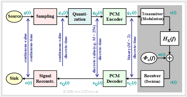
$q(t)\ \circ\!\!-\!\!\!-\!\!\!-\!\!\bullet\,\ Q(f)$ ⇒ source signal (from German: "Quellensignal"), analog
$q_{\rm A}(t)\ \circ\!\!-\!\!\!-\!\!\!-\!\!\bullet\,\ Q_{\rm A}(f)$ ⇒ sampled source signal (from German: "abgetastet" ⇒ "A")
$q_{\rm Q}(t)\ \circ\!\!-\!\!\!-\!\!\!-\!\!\bullet\,\ Q_{\rm Q}(f)$ ⇒ quantized source signal (from German: "quantisiert" ⇒ "Q")
$q_{\rm C}(t)\ \circ\!\!-\!\!\!-\!\!\!-\!\!\bullet\,\ Q_{\rm C}(f)$ ⇒ coded source signal (from German: "codiert" ⇒ "C"), binary
$s(t)\ \circ\!\!-\!\!\!-\!\!\!-\!\!\bullet\,\ S(f)$ ⇒ transmitted signal (from German: "Sendesignal"), digital
$n(t)$ ⇒ noise signal, characterized by the power-spectral density ${\it Φ}_n(f)$, analog $r(t)= s(t) \star h_{\rm K}(t) + n(t)$ ⇒ received signal, $h_{\rm K}(t)\ \circ\!\!-\!\!\!-\!\!\!-\!\!\bullet\,\ H_{\rm K}(f)$, analog
Note: Spectrum $R(f)$ can not be specified due to the stochastic component $n(t)$.
$v_{\rm C}(t)\ \circ\!\!-\!\!\!-\!\!\!-\!\!\bullet\,\ V_{\rm C}(f)$ ⇒ signal after decision, binary
$v_{\rm Q}(t)\ \circ\!\!-\!\!\!-\!\!\!-\!\!\bullet\,\ V_{\rm Q}(f)$ ⇒ signal after PCM decoding, $M$–level
Note: On the receiver side, there is no counterpart to "Quantization"
$v(t)\ \circ\!\!-\!\!\!-\!\!\!-\!\!\bullet\,\ V(f)$ ⇒ sink signal, analog
Further it should be noted to this PCM block diagram:
- The PCM transmitter ("A/D converter") is composed of three function blocks »Sampling - Quantization - PCM Coding« which will be described in more detail in the next sections.
- The gray-background block "Digital Transmission System" shows "transmitter" (modulation), "receiver" (with decision unit), and "analog transmission channel" ⇒ channel frequency response $H_{\rm K}(f)$ and noise power-spectral density ${\it Φ}_n(f)$.
- This block is covered in the first three chapters of the book "Digital Signal Transmission". In chapter 5 of the same book, you will find $\text{digital channel models}$ that phenomenologically describe the transmission behavior using the signals $q_{\rm C}(t)$ and $v_{\rm C}(t)$.
- Further, it can be seen from the block diagram that there is no equivalent for "quantization" at the receiver-side. Therefore, even with error-free transmission, i.e., for $v_{\rm C}(t) = q_{\rm C}(t)$, the analog sink signal $v(t)$ will differ from the source signal $q(t)$.
- As a measure of the quality of the digital transmission system, we use the $\text{Signal-to-Noise Power Ratio}$ ⇒ in short: »Sink-SNR« as the quotient of the powers of source signal $q(t)$ and error signal $ε(t) = v(t) - q(t)$:
- $$\rho_{v} = \frac{P_q}{P_\varepsilon}\hspace{0.3cm} {\rm with}\hspace{0.3cm}P_q = \overline{[q(t)]^2}, \hspace{0.2cm}P_\varepsilon = \overline{[v(t) - q(t)]^2}\hspace{0.05cm}.$$
- Here, an ideal amplitude matching is assumed, so that in the ideal case (that is: sampling according to the sampling theorem, best possible signal reconstruction, infinitely fine quantization) the sink signal $v(t)$ would exactly match the source signal $q(t)$.
⇒ We would like to refer you already here to the three-part (German language) learning video "Pulse Code Modulation" which contains all aspects of PCM. Its principle is explained in detail in the first part of the video.
Sampling and signal reconstruction
Sampling – that is, time discretization of the analog signal $q(t)$ – was covered in detail in the chapter "Discrete-Time Signal Representation" of the book "Signal Representation." Here follows a brief summary of that section.
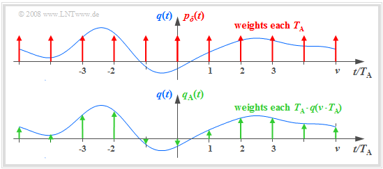
The graph illustrates the sampling in the time domain:
- The (blue) source signal $q(t)$ is "continuous-time", the (green) signal sampled at a distance $T_{\rm A}$ is "discrete-time".
- The sampling can be represented by multiplying the analog signal $q(t)$ by the $\text{Dirac comb in the time domain}$ ⇒ $p_δ(t)$:
- $$q_{\rm A}(t) = q(t) \cdot p_{\delta}(t)\hspace{0.3cm} {\rm with}\hspace{0.3cm}p_{\delta}(t)= \sum_{\nu = -\infty}^{\infty}T_{\rm A}\cdot \delta(t - \nu \cdot T_{\rm A}) \hspace{0.05cm}.$$
- The Dirac delta function at $t = ν \cdot T_{\rm A}$ has the weight $T_{\rm A} \cdot q(ν \cdot T_{\rm A})$. Since $δ(t)$ has the unit "$\rm 1/s$" thus $q_{\rm A}(t)$ has the same unit as $q(t)$, e.g. "V".
- The Fourier transform of the Dirac comb $p_δ(t)$ is also a Dirac comb, but now in the frequency domain ⇒ $P_δ(f)$. The spacing of the individual Dirac delta lines is $f_{\rm A} = 1/T_{\rm A}$, and all weights of $P_δ(f)$ are $1$:
- $$p_{\delta}(t)= \sum_{\nu = -\infty}^{+\infty}T_{\rm A}\cdot \delta(t - \nu \cdot T_{\rm A}) \hspace{0.2cm}\circ\!\!-\!\!\!-\!\!\!-\!\!\bullet\, \hspace{0.2cm} P_{\delta}(f)= \sum_{\mu = -\infty}^{+\infty} \delta(f - \mu \cdot f_{\rm A}) \hspace{0.05cm}.$$
- The spectrum $Q_{\rm A}(f)$ of the sampled source signal $q_{\rm A}(t)$ is obtained from the $\text{Convolution Theorem}$, where $Q(f)\hspace{0.2cm}\bullet\!\!-\!\!\!-\!\!\!-\!\!\circ\, \hspace{0.2cm} q(t):$
- $$Q_{\rm A}(f) = Q(f) \star P_{\delta}(f)= \sum_{\mu = -\infty}^{+\infty} Q(f - \mu \cdot f_{\rm A}) \hspace{0.05cm}.$$
⇒ We refer you to part 2 of the (German language) learning video "Pulse Code Modulation" which explains sampling and signal reconstruction in terms of system theory.
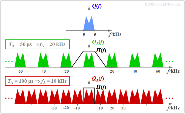
$\text{Example 1:}$ The graph schematically shows the spectrum $Q(f)$ of an analog source signal $q(t)$ with frequencies up to $f_{\rm N, \ max} = 5 \ \rm kHz$.
- If one samples $q(t)$ with the sampling rate $f_{\rm A} = 20 \ \rm kHz$ $($so at the respective distance $T_{\rm A} = 50 \ \rm µ s)$, one obtains the periodic spectrum $Q_{\rm A}(f)$ sketched in green.
- Since the Dirac delta functions are infinitely narrow, $q_{\rm A}(t)$ also contains arbitrary high frequency components and accordingly $Q_{\rm A}(f)$ is extended to infinity (middle graph).
- Drawn below (in red) is the spectrum $Q_{\rm A}(f)$ of the sampled source signal for the sampling parameters $T_{\rm A} = 100 \ \rm µ s$ ⇒ $f_{\rm A} = 10 \ \rm kHz$.
$\text{Conclusion:}$ From this example, the following important lessons can be learned regarding sampling:
- If $Q(f)$ contains frequencies up to $f_\text{N, max}$, then according to the $\text{Sampling Theorem}$ the sampling rate $f_{\rm A} ≥ 2 \cdot f_\text{N, max}$ should be chosen. At smaller sampling rate $f_{\rm A}$ $($thus larger spacing $T_{\rm A})$ overlaps of the periodized spectra occur, i.e. irreversible distortions.
- If exactly $f_{\rm A} = 2 \cdot f_\text{N, max}$ as in the lower graph of $\text{Example 1}$, then $Q(f)$ can be can be completely reconstructed from $Q_{\rm A}(f)$ by an ideal rectangular low-pass filter $H(f)$ with cutoff frequency $f_{\rm G} = f_{\rm A}/2$. The same facts apply in the $\text{PCM system}$ to extract $V(f)$ from $V_{\rm Q}(f)$ in the best possible way.
- On the other hand, if sampling is performed with $f_{\rm A} > 2 \cdot f_\text{N, max}$ as in the middle graph of the example, a low-pass filter $H(f)$ with a smaller slope can also be used on the receiver side for signal reconstruction, as long as the following condition is met:
- $$H(f) = \left\{ \begin{array}{l} 1 \\ 0 \\ \end{array} \right.\quad \begin{array}{*{5}c}{\rm{for} } \\{\rm{for} } \\ \end{array}\begin{array}{*{10}c} {\hspace{0.04cm}\left \vert \hspace{0.005cm} f\hspace{0.05cm} \right \vert \le f_{\rm N, \hspace{0.05cm}max},} \\ {\hspace{0.04cm}\left \vert\hspace{0.005cm} f \hspace{0.05cm} \right \vert \ge f_{\rm A}- f_{\rm N, \hspace{0.05cm}max}.} \\ \end{array}$$
Natural and discrete sampling
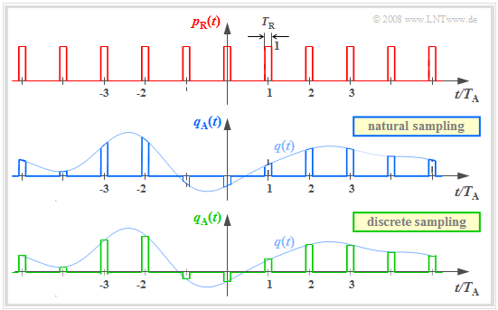
Multiplication by the Dirac comb provides only an idealized description of the sampling, since a Dirac delta function $($duration $T_{\rm R} → 0$, height $1/T_{\rm R} → ∞)$ is not realizable. In practice, the "Dirac comb" $p_δ(t)$ must be replaced by a "rectangular pulse comb" $p_{\rm R}(t)$ with rectangle duration $T_{\rm R}$ (see upper sketch):
- $$p_{\rm R}(t)= \sum_{\nu = -\infty}^{+\infty}g_{\rm R}(t - \nu \cdot T_{\rm A}),$$
- $$g_{\rm R}(t) = \left\{ \begin{array}{l} 1 \\ 1/2 \\ 0 \\ \end{array} \right.\quad \begin{array}{*{5}c}{\rm{for}}\\{\rm{for}} \\{\rm{for}} \\ \end{array}\begin{array}{*{10}c}{\hspace{0.04cm}\left|\hspace{0.06cm} t \hspace{0.05cm} \right|} < T_{\rm R}/2\hspace{0.05cm}, \\{\hspace{0.04cm}\left|\hspace{0.06cm} t \hspace{0.05cm} \right|} = T_{\rm R}/2\hspace{0.05cm}, \\ {\hspace{0.005cm}\left|\hspace{0.06cm} t \hspace{0.05cm} \right|} > T_{\rm R}/2\hspace{0.05cm}. \\ \end{array}$$
$T_{\rm R}$ should be significantly smaller than the sampling distance $T_{\rm A}$.
The graphic show two different sampling methods using the comb $p_{\rm R}(t)$:
- In »natural sampling« the sampled signal $q_{\rm A}(t)$ is obtained by multiplying the analog source signal $q(t)$ by $p_{\rm R}(t)$. Thus in the ranges $p_{\rm R}(t) = 1$, $q_{\rm A}(t)$ has the same progression as $q(t)$.
- In »discrete sampling« the signal $q(t)$ is – at least mentally – first multiplied by the Dirac comb $p_δ(t)$. Then each Dirac delta pulse $T_{\rm A} \cdot δ(t - ν \cdot T_{\rm A})$ is replaced by a rectangular pulse $g_{\rm R}(t - ν \cdot T_{\rm A})$ .
Here and in the following frequency domain consideration, an acausal description form is chosen for simplicity.
For a (causal) realization, $g_{\rm R}(t) = 1$ would have to hold in the range from $0$ to $T_{\rm R}$ and not as here for $ -T_{\rm R}/2 < t < T_{\rm R}/2.$
Frequency domain view of natural sampling
$\text{Definition:}$ The »natural sampling« can be represented by the convolution theorem in the spectral domain as follows:
- $$q_{\rm A}(t) = p_{\rm R}(t) \cdot q(t) = \left [ \frac{1}{T_{\rm A} } \cdot p_{\rm \delta}(t) \star g_{\rm R}(t)\right ]\cdot q(t) \hspace{0.3cm} \Rightarrow \hspace{0.3cm}Q_{\rm A}(f) = \left [ P_{\rm \delta}(f) \cdot \frac{1}{T_{\rm A} } \cdot G_{\rm R}(f) \right ] \star Q(f) = P_{\rm R}(f) \star Q(f)\hspace{0.05cm}.$$
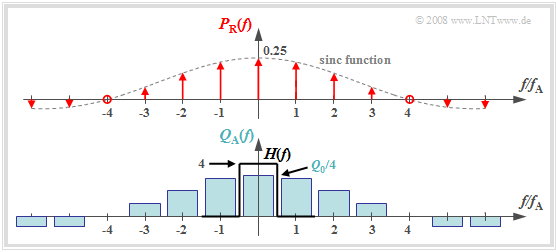
The graph shows the result for
- an (unrealistic) rectangular spectrum $Q(f) = Q_0$ limited to the range $|f| ≤ 4 \ \rm kHz$,
- the sampling rate $f_{\rm A} = 10 \ \rm kHz$ ⇒ $T_{\rm A} = 100 \ \rm µ s$, and
- the rectangular pulse duration $T_{\rm R} = 25 \ \rm µ s$ ⇒ $T_{\rm R}/T_{\rm A} = 0.25$.
One can see from this plot:
- The spectrum $P_{\rm R}(f)$ is in contrast to $P_δ(f)$ not a Dirac comb $($all weights equal $1)$, but the weights here are evaluated to the function $G_{\rm R}(f)/T_{\rm A} = T_{\rm R}/T_{\rm A} \cdot {\rm sinc}(f\cdot T_{\rm R})$.
- Because of the zero of the $\rm sinc$-function, the Dirac delta lines vanish here at $±4f_{\rm A}$.
- The spectrum $Q_{\rm A}(f)$ results from the convolution with $Q(f)$. The rectangle around $f = 0$ has height $T_{\rm R}/T_{\rm A} \cdot Q_0$, the proportions around $\mu \cdot f_{\rm A} \ (\mu ≠ 0)$ are lower.
- If one uses for signal reconstruction an ideal, rectangular low-pass
- $$H(f) = \left\{ \begin{array}{l} T_{\rm A}/T_{\rm R} = 4 \\ 0 \\ \end{array} \right.\quad \begin{array}{*{5}c}{\rm{for}}\\{\rm{for}} \\ \end{array}\begin{array}{*{10}c} {\hspace{0.04cm}\left| \hspace{0.005cm} f\hspace{0.05cm} \right| < f_{\rm A}/2}\hspace{0.05cm}, \\ {\hspace{0.04cm}\left| \hspace{0.005cm} f\hspace{0.05cm} \right| > f_{\rm A}/2}\hspace{0.05cm}, \\ \end{array},$$
- then for the output spectrum $V(f) = Q(f)$ ⇒ $v(t) = q(t)$.
$\text{Conclusion:}$
- For natural sampling, a rectangular–low-pass filter is sufficient for signal reconstruction as for ideal sampling (with Dirac comb).
- However, for amplitude matching in the passband, a gain by the factor $T_{\rm A}/T_{\rm R}$ must be considered.
Frequency domain view of discrete sampling
$\text{Definition:}$ In »discrete sampling« the multiplication of the Dirac comb $p_δ(t)$ with the source signal $q(t)$ takes place first – at least mentally – and only afterwards the convolution with the rectangular pulse $g_{\rm R}(t)$:
- $$q_{\rm A}(t) = \big [ {1}/{T_{\rm A} } \cdot p_{\rm \delta}(t) \cdot q(t)\big ]\star g_{\rm R}(t) \hspace{0.3cm} \Rightarrow \hspace{0.3cm}Q_{\rm A}(f) = \big [ P_{\rm \delta}(f) \star Q(f) \big ] \cdot G_{\rm R}(f)/{T_{\rm A} } \hspace{0.05cm}.$$
- It is irrelevant, but quite convenient, that here the factor $1/T_{\rm A}$ has been added to the evaluation function $G_{\rm R}(f)$.
- Thus, $G_{\rm R}(f)/T_{\rm A} = T_{\rm R}/T_{\rm A} \cdot {\rm sinc}(fT_{\rm R}).$
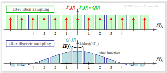
- The upper graph shows (highlighted in green) the spectral function $P_δ(f) \star Q(f)$ after ideal sampling.
- In contrast, discrete sampling with a rectangular comb yields the spectrum $Q_{\rm A}(f)$ corresponding to the lower graph.
You can see from this plot:
- Each of the infinitely many partial spectra now has a different shape. Only the middle spectrum around $f = 0$ is important;
- All other spectral components are removed at the receiver side by the low-pass of the signal reconstruction.
- If one uses for this low-pass again a rectangular filter with the gain $T_{\rm A}/T_{\rm R}$ in the passband, one obtains for the output spectrum:
- $$V(f) = Q(f) \cdot {\rm sinc}(f \cdot T_{\rm R}) \hspace{0.05cm}.$$
$\text{Conclusion:}$ Discrete sampling and rectangular filtering result in attenuation distortions according to the weighting function ${\rm sinc}(f \cdot T_{\rm R})$.
- These are stronger, the larger $T_{\rm R}$ is. Only in the limiting case $T_{\rm R} → 0$ holds ${\rm sinc}(f\cdot T_{\rm R}) = 1$.
- However, ideal equalization can fully compensate for these linear attenuation distortions. To obtain $V(f) = Q(f)$ resp. $v(t) = q(t)$ then must hold:
- $$H(f) = \left\{ \begin{array}{l} (T_{\rm A}/T_{\rm R})/{\rm sinc}(f \cdot T_{\rm R}) \\ 0 \\ \end{array} \right.\quad\begin{array}{*{5}c}{\rm{for} }\\{\rm{for} } \\ \end{array}\begin{array}{*{10}c} {\hspace{0.04cm}\left \vert \hspace{0.005cm} f\hspace{0.05cm} \right \vert < f_{\rm A}/2}\hspace{0.05cm}, \\ {\hspace{0.04cm}\left \vert \hspace{0.005cm} f\hspace{0.05cm} \right \vert > f_{\rm A}/2.} \\ \end{array}$$
Quantization and quantization noise
The second functional unit »Quantization« of the PCM transmitter is used for value discretization.
- For this purpose the whole value range of the analog source signal $($e.g., the range $± q_{\rm max})$ is divided into $M$ intervals.
- Each sample $q_{\rm A}(ν ⋅ T_{\rm A})$ is then assigned to a representative $q_{\rm Q}(ν ⋅ T_{\rm A})$ of the associated interval (e.g., the interval center) .
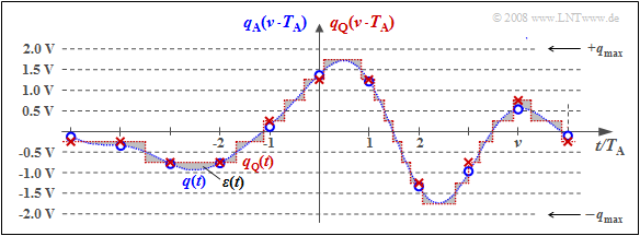
$\text{Example 2:}$ The graph illustrates the unit "quantization" using the quantization step number $M = 8$ as an example.
- In fact, a power of two is always chosen for $M$ in practice because of the subsequent binary coding.
- Each of the samples $q_{\rm A}(ν \cdot T_{\rm A})$ marked by circles is replaced by the corresponding quantized value $q_{\rm Q}(ν \cdot T_{\rm A})$. The quantized values are entered as crosses.
- However, this process of value discretization is associated with an irreversible falsification.
- The falsification $ε_ν = q_{\rm Q}(ν \cdot T_{\rm A}) \ - \ q_{\rm A}(ν \cdot T_{\rm A})$ depends on the quantization level number $M$. The following bound applies:
- $$\vert \varepsilon_{\nu} \vert < {1}/{2} \cdot2/M \cdot q_{\rm max}= {q_{\rm max} }/{M}\hspace{0.05cm}.$$
$\text{Definition:}$ One refers to the second moment of the error quantity $ε_ν$ as »quantization noise power«:
- $$P_{\rm Q} = \frac{1}{2N+1 } \cdot\sum_{\nu = -N}^{+N}\varepsilon_{\nu}^2 \approx \frac{1}{N \cdot T_{\rm A} } \cdot \int_{0}^{N \cdot T_{\rm A} }\varepsilon(t)^2 \hspace{0.05cm}{\rm d}t \hspace{0.3cm} {\rm with}\hspace{0.3cm}\varepsilon(t) = q_{\rm Q}(t) - q(t) \hspace{0.05cm}.$$
Notes:
- For calculating the quantization noise power $P_{\rm Q}$ the given approximation of "spontaneous quantization" is usually used.
- Here, one ignores sampling and forms the error signal from the continuous-time signals $q_{\rm Q}(t)$ and $q(t)$.
- $P_{\rm Q}$ also depends on the source signal $q(t)$. Assuming that $q(t)$ takes all values between $±q_{\rm max}$ with equal probability and the quantizer is designed exactly for this range, we get accordingly "Exercise 4.4":
- $$P_{\rm Q} = \frac{q_{\rm max}^2}{3 \cdot M^2 } \hspace{0.05cm}.$$
- In a speech or music signal, arbitrarily large amplitude values can occur - even if only very rarely. In this case, for $q_{\rm max}$ usually that amplitude value is used which is exceeded (in amplitude) only at $1\%$ all times.
PCM encoding and decoding
The block »PCM coding« is used to convert the discrete-time (after sampling) and discrete-value (after quantization with $M$ steps) signal values $q_{\rm Q}(ν - T_{\rm A})$ into a sequence of $N = {\rm log_2}(M)$ binary values. Logarithm to base 2 ⇒ "binary logarithm".
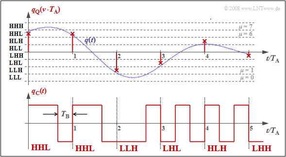
$\text{Example 3:}$ Each binary value ⇒ bit is represented by a rectangle of duration $T_{\rm B} = T_{\rm A}/N$ resulting in the signal $q_{\rm C}(t)$. You can see:
- Here, the "dual code" is used ⇒ the quantization intervals $\mu$ are numbered consecutively from $0$ to $M-1$ and then written in simple binary. With $M = 8$ for example $\mu = 6$ ⇔ 110.
- The three symbols of the binary encoded signal $q_{\rm C}(t)$ are obtained by replacing 0 by L ("Low") and 1 by H ("High"). This gives in the example the sequence "HHL HHL LLH LHL HLH LHH".
- The bit duration $T_{\rm B}$ is here shorter than the sampling distance $T_{\rm A} = 1/f_{\rm A}$ by a factor $N = {\rm log_2}(M) = 3$. So, the bit rate is $R_{\rm B} = {\rm log_2}(M) \cdot f_{\rm A}$.
- If one uses the same mapping in decoding $(v_{\rm C} ⇒ v_{\rm Q})$ as in encoding $(q_{\rm Q} ⇒ q_{\rm C})$, then, if there are no transmission errors: $v_{\rm Q}(ν \cdot T_{\rm A}) = q_{\rm Q}(ν \cdot T_{\rm A}). $
- An alternative to dual code is "Gray code", where adjacent binary values differ only in one bit. For $N = 3$:
- $\mu = 0$: LLL, $\mu = 1$: LLH, $\mu = 2$: LHH, $\mu = 3$: LHL,
- $\mu = 4$: HHL, $\mu = 5$: HHH, $\mu =6$: HLH, $\mu = 7$: HLL.
Signal-to-noise power ratio
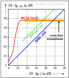
The digital "pulse code modulation" $\rm (PCM)$ is now compared to analog modulation methods $\rm (AM, \ FM)$ regarding the achievable sink SNR $ρ_v = P_q/P_ε$ with AWGN noise. As denoted in previous chapters $\text{(for example)}$ $ξ = {α_{\rm K}}^2 \cdot P_{\rm S}/(N_0 \cdot B_{\rm NF})$ the "performance parameter" $ξ$ summarizes different influences:
- The channel transmission factor $α_{\rm K}$ (quadratic),
- the transmit power $P_{\rm S}$ (linear),
- the AWGN noise power density $N_0$ (reciprocal), and.
- the signal bandwidth $B_{\rm NF}$ (reciprocal); for a harmonic oscillation: signal frequency $f_{\rm N}$ instead of $B_{\rm NF}$.
The two comparison curves for $\text{amplitude modulation}$ and $\text{frequency modulation}$ can be described as follows:
- Double-sideband amplitude modulation $\text{(DSB–AM)}$ without carrier $(m \to \infty)$:
- $$ρ_v = ξ \ ⇒ \ 10 · \lg ρ_v = 10 · \lg \ ξ.$$
- Frequency modulation $\text{(FM)}$ with modulation index $η = 3$:
- $$ρ_υ = 3/2 \cdot η^2 - ξ = 13.5 - ξ \ ⇒ \ 10 · \lg \ ρ_v = 10 · \lg \ ξ + 11.3 \ \rm dB.$$
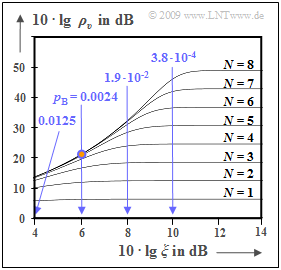
The curve for the $\text{PCM 30/32}$ system should be interpreted as follows:
- If the performance parameter $ξ$ is sufficiently large, then no transmission errors occur. The error signal $ε(t) = v(t) \ - \ q(t)$ is then alone due to quantization $(P_ε = P_{\rm Q})$.
- With the quantization step number $M = 2^N$ holds approximately in this case:
- $$\rho_{v} = \frac{P_q}{P_\varepsilon}= M^2 = 2^{2N} \hspace{0.3cm}\Rightarrow \hspace{0.3cm} 10 \cdot {\rm lg}\hspace{0.1cm}\rho_{v}=20 \cdot {\rm lg}\hspace{0.1cm}M = N \cdot 6.02\,{\rm dB}$$
- $$ \Rightarrow \hspace{0.3cm} N = 8, \hspace{0.05cm} M =256\text{:}\hspace{0.2cm}10 \cdot {\rm lg}\hspace{0.1cm}\rho_{v}=48.16\,{\rm dB}\hspace{0.05cm}.$$
- Note that the given equation is exactly valid only for a sawtooth shaped source signal. However, for a cosine shaped signal the deviation from this is not very large.
- As $ξ$ decreases (smaller transmit power or larger noise power density), the transmission errors increase. Thus $P_ε > P_{\rm Q}$ and the sink-to-noise ratio becomes smaller.
- PCM $($with $M = 256)$ is superior to the analog methods $($AM and FM$)$ only in the lower and middle $ξ$–range. But if transmission errors do not play a role anymore, no improvement can be achieved by a larger $ξ$ $($horizontal curve section with yellow background$)$.
- An improvement is only achieved by increasing $N$ $($number of bits per sample$)$ ⇒ larger $M = 2^N$ $($number of quantization steps$)$. For example, for a »Compact Disc« $\rm (CD)$ with parameter $N = 16$ ⇒ $M = 65536$ the sink SNR is:
- $$10 · \lg \ ρ_v = 96.32 \ \rm dB.$$
$\text{Example 4:}$ The following graph shows the limiting influence of quantization:
- Here, transmission errors are excluded. Sampling and signal reconstruction are best fit to $q(t)$.
- White dotted is the source signal $q(t)$, green dotted is the sink signal $v(t)$ after PCM with $N = 4$ ⇒ $M = 16$.
- Sampling times are marked by crosses.
This image can be interpreted as follows:
- With $N = 8$ ⇒ $M = 256$ the sink signal $v(t)$ cannot be distinguished with the naked eye from the source signal $q(t)$. The white dotted signal curve applies approximately to both.
- But from the signal-to-noise ratio $10 · \lg \ ρ_v = 47.8 \ \rm dB$ it can be seen that the quantization noise power $P_\varepsilon$ is only smaller by a factor $1. 6 \cdot 10^{-5}$ than the power $P_q$ of the source signal.
- This SNR would already be clearly audible with a speech or music signal.
- Although $q(t)$ is neither sawtooth nor cosine shaped, but is composed of several frequency components, the approximation $ρ_v ≈ M^2$ ⇒ $10 · \lg \ ρ_υ = 48.16 \ \rm dB$ deviates insignificantly from the actual value.
- In contrast, for $N = 4$ ⇒ $M = 16$ the deviations between sink signal (marked in green) and source signal (marked in white) can already be seen in the image, which is also quantitatively expressed by the very small SNR $10 · \lg \ ρ_υ = 28.2 \ \rm dB$.
Influence of transmission errors
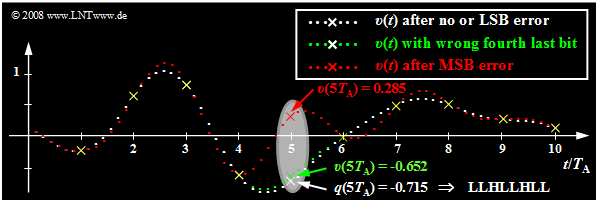
Starting from the same analog signal $q(t)$ as in the last section and a linear quantization with $N = 8$ bits ⇒ $M = 256$ the effects of transmission errors are now illustrated using the respective sink signal $v(t)$.
- The white dots mark the source signal $q(t)$. Without transmission error the sink signal $v(t)$ has the same course when neglecting quantization.
- Now, exactly one bit of the fifth sample $q(5 \cdot T_{\rm A}) = -0.715$ is falsified, where this sample has been encoded as LLHL LHLL.
The results of the error analysis shown in the graph and the table below can be summarized as follows:
- If only the last bit ⇒ "Least Significant Bit" ⇒ $\rm (LSB)$ of the binary word is falsified $($LLHL LHLL ⇒ LLHL LHLH, white curve$)$, then no difference from error-free transmission is visible to the naked eye. Nevertheless, the signal-to-noise ratio is reduced by $3.5 \ \rm dB$.
- An error of the fourth last bit leads to a clearly detectable distortion by eight quantization steps $($LLHLLHLL ⇒ LLHLHHLL, green curve$)$: $v(5T_{\rm A}) \ - \ q(5T_{\rm A}) = 8/256 - 2 = 0.0625$ and the signal-to-noise ratio drops to $10 · \lg \ ρ_υ = 28.2 \ \rm dB$.
- Finally, the red curve shows the case where the $\rm MSB$ ("Most Significant Bit") is falsified: LLHLLHLL ⇒ HLHLLHLL ⇒ distortion $v(5T_{\rm A}) \ - \ q(5T_{\rm A}) = 1$ $($corresponding to half the modulation range$)$. The SNR is now only about $4 \ \rm dB$.
- At all sampling times except $5T_{\rm A}$, $v(t)$ matches exactly with $q(t)$ except for the quantization error. Outside these points marked by yellow crosses, the single error at $5T_{\rm A}$ leads to strong deviations in an extended range, due to the interpolation with the $\rm sinc$-shaped impulse response of the reconstruction low-pass $H(f)$.
Estimation of SNR degradation due to transmission errors
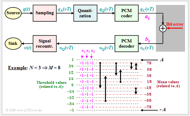
Now we will try to (approximately) determine the SNR curve of the PCM system taking bit errors into account. We start from the following block diagram and further assume:
- Each sample $q_{\rm A}(νT)$ is quantized by $M$ steps and represented by $N = {\rm log_2} (M)$ bits. In the example: $M = 8$ ⇒ $N = 3$.
- The binary representation of $q_{\rm Q}(νT)$ yields the coefficients $a_k\, (k = 1, \text{...} \hspace{0.08cm}, N)$, which can be falsified by bit errors to the coefficients $b_k$. Both $a_k$ and $b_k$ are $±1$, respectively.
- A bit error $(b_k ≠ a_k)$ occurs with probability $p_{\rm B}$. Each bit is equally likely to be falsified and in each PCM word there is at most one error ⇒ only one of the $N$ bits can be wrong.
From the diagram given in the graph, it can be seen for $N = 3$ and natural binary coding ("Dual Code"):
- A falsification of $a_1$ changes the value $q_{\rm Q}(νT)$ by $±A$.
- A falsification of $a_2$ changes the value $q_{\rm Q}(νT)$ by $±A/2$.
- A falsification of $a_3$ changes the value value $q_{\rm Q}(νT)$ by $±A/4$.
For the case when (only) the coefficient $a_k$ was falsified, we obtain by generalization for the deviation:
- $$\varepsilon_k = υ_{\rm Q}(νT) \ - \ q_{\rm Q}(νT)= - a_k \cdot A \cdot 2^{-k +1} \hspace{0.05cm}.$$
After averaging over all falsification values $ε_k$ (with $1 ≤ k ≤ N)$ taking into account the bit error probability $p_{\rm B}$ we obtain for the "error noise power":
- $$P_{\rm E}= {\rm E}\big[\varepsilon_k^2 \big] = \sum\limits^{N}_{k = 1} p_{\rm B} \cdot \left ( - a_k \cdot A \cdot 2^{-k +1} \right )^2 =\ p_{\rm B} \cdot A^2 \cdot \sum\limits^{N-1}_{k = 0} 2^{-2k } = p_{\rm B} \cdot A^2 \cdot \frac{1- 2^{-2N }}{1- 2^{-2 }} \approx {4}/{3} \cdot p_{\rm B} \cdot A^2 \hspace{0.05cm}.$$
- Here are used the sum formula of the geometric series and the approximation $1 - 2^{-2N } ≈ 1$.
- For $N = 8$ ⇒ $M = 256$ the associated relative error is about $\rm 10^{-5}$.
Excluding transmission errors, the signal-to-noise power ratio $ρ_v = P_{\rm S}/P_{\rm Q}$ has been found, where for a uniformly distributed source signal $($e.g. sawtooth-shaped$)$ the signal power and quantization noise power are to be calculated as follows:
- $$P_{\rm S}={A^2}/{3}\hspace{0.05cm},\hspace{0.3cm}P_{\rm Q}= {A^2}/{3} \cdot 2^{-2N } \hspace{0.05cm}.$$
Taking into account the transmission errors, the above result gives:
- $$\rho_{\upsilon}= \frac{P_{\rm S}}{P_{\rm Q}+P_{\rm E}} = \frac{A^2/3}{A^2/3 \cdot 2^{-2N } + A^2/3 \cdot 4 \cdot p_{\rm B}} = \frac{1}{ 2^{-2N } + 4 \cdot p_{\rm B}} \hspace{0.05cm}.$$
The graph shows $10 \cdot \lg ρ_v$ as a function of the (logarithmized) power parameter $ξ = P_{\rm S}/(N_0 \cdot B_{\rm NF})$, where $B_{\rm NF}$ indicates the source signal bandwidth. Let the constant channel transmission factor be ideally $α_{\rm K} = 1$. Then holds:
- For AWGN noise and the optimum binary system, the performance parameter is also $ξ = E_{\rm B}/N_0$ $($energy per bit related to noise power density$)$. The bit error probability is then given by the Gaussian error function ${\rm Q}(x)$:
- $$p_{\rm B}= {\rm Q} \left ( \sqrt{{2E_{\rm B}}/{N_0} }\right ) \hspace{0.05cm}.$$
- For $N = 8$ ⇒ $ 2^{-2{\it N} } = 1.5 \cdot 10^{-5}$ and $10 \cdot \lg \ ξ = 6 \ \rm dB$ ⇒ $p_{\rm B} = 0.0024$ $($point marked in red$)$ results:
- $$\rho_{\upsilon}= \frac{1}{ 1.5 \cdot 10^{-5} + 4 \cdot 0.0024} \approx 100 \hspace{0.3cm} \Rightarrow \hspace{0.3cm}10 \cdot {\rm lg} \hspace{0.15cm}\rho_{\upsilon}\approx 20\,{\rm dB} \hspace{0.05cm}.$$
- This small $ρ_v$ value goes back to the term $4 · 0.0024$ in the denominator $($influence of the transmission errors$)$ while in the horizontal section of the curve for each $N$ (number of bits per sample) the term $\rm 2^{-2{\it N} }$ dominates - i.e. the quantization noise.
Non-linear quantization
Often the quantization intervals are not chosen equally large, but one uses a finer quantization for the inner amplitude range than for large amplitudes. There are several reasons for this:
- In audio signals, distortions of the quiet signal components (i.e. values near the zero line) are subjectively perceived as more disturbing than an impairment of large amplitude values.
- Such an uneven quantization also leads to a larger sink SNR for such a music or speech signal, because here the signal amplitude is not uniformly distributed.
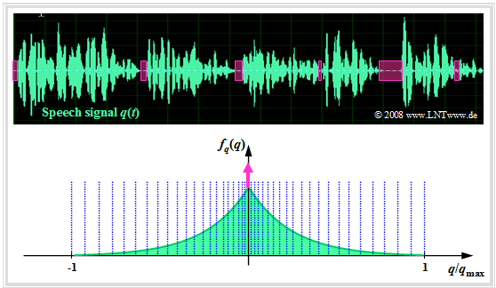
The graph shows a speech signal $q(t)$ and its amplitude distribution $f_q(q)$ ⇒ $\text{Probability density function}$ $\rm (PDF)$.
This is the $\text{Laplace distribution}$, which can be approximated as follows:
- by a continuous-valued two-sided exponential distribution, and
- by a Dirac delta function $δ(q)$ to account for the speech pauses (magenta colored).
In the graph, nonlinear quantization is only implied, e.g. by means of the 13-segment characteristic, which is described in more detail in the "Exercise 4.5" :
- The quantization intervals here become wider and wider towards the edges section by section.
- The more frequent small amplitudes, on the other hand, are quantized very finely.
Compression and expansion
Non-uniform quantization can be realized, for example, by
- the sampled values $q_{\rm A}(ν \cdot T_{\rm A})$ are first deformed by a nonlinear characteristic $q_{\rm K}(q_{\rm A})$, and
- subsequently, the resulting output values $q_{\rm K}(ν · T_{\rm A})$ are uniformly quantized.
This results in the signal chain sketched on the right.
$\text{Conclusion:}$ Such a non-uniform quantization means:
- Through the nonlinear characteristic $q_{\rm K}(q_{\rm A})$ ⇒ small signal values are amplified and large values are attenuated ⇒ »compression«.
- This deliberate signal distortion is undone at the receiver by the inverse function $v_{\rm E}(υ_{\rm Q})$ ⇒ »expansion«.
- The total process of transmitter-side compression and receiver-side expansion is also called »companding.«
For the PCM system 30/32, the "Comité Consultatif International des Télégraphique et Téléphonique" $\rm (CCITT)$ recommended the so-called "A–characteristic":
- $$y(x) = \left\{ \begin{array}{l} \frac{1 + {\rm ln}(A \cdot x)}{1 + {\rm ln}(A)} \\ \frac{A \cdot x}{1 + {\rm ln}(A)} \\ - \frac{1 + {\rm ln}( - A \cdot x)}{1 + {\rm ln}(A)} \\ \end{array} \right.\quad\begin{array}{*{5}c}{\rm{for}}\\{\rm{for}}\\{\rm{for}} \\ \end{array}\begin{array}{*{10}c}1/A \le x \le 1\hspace{0.05cm}, \\ - 1/A \le x \le 1/A\hspace{0.05cm}, \\ - 1 \le x \le - 1/A\hspace{0.05cm}. \\ \end{array}$$
- Here, for abbreviation $x = q_{\rm A}(ν \cdot T_{\rm A})$ and $y = q_{\rm K}(ν \cdot T_{\rm A})$ are used.
- This characteristic curve with the value $A = 87.56$ introduced in practice has a constantly changing slope.
- For more details on this type of non-uniform quantization, see the "Exercise 4.6".
⇒ Note: In the third part of the (German language) learning video "Pulse Code Modulation" are covered:
- the definition of signal-to-noise power ratio $\rm (SNR)$,
- the influence of quantization noise and transmission errors,
- the differences between linear and non-linear quantization.
Exercises for the chapter
Exercise 4.1: PCM System 30/32
Exercise 4.2: Low-Pass for Signal Reconstruction
Exercise 4.2Z: About the Sampling Theorem
Exercise 4.3: Natural and Discrete Sampling
Exercise 4.4: About the Quantization Noise
Exercise 4.4Z: Signal-to-Noise Ratio with PCM
Exercise 4.5: Non-Linear Quantization
Exercise 4.6: Quantization Characteristics
